Interest in fundamental tax reform has waned since the early months of the 1996 U.S. presidential campaign when it was the subject of intense political and media debate. In coming years, a resurgence of interest seems almost cer-tain. After all, the Internal Revenue Service remains unpopular, the U.S. savings rate re-mains low, and pressure to efficiently raise sub-stantial new tax revenues will grow once the baby boom generation reaches retirement age and federal entitlement spending begins to bal-loon. Now, while the rhetoric is still somewhat subdued, may be a good time to review the impact a major tax overhaul would have on the economy.
In this first of two articles on the economic impact of fundamental tax reform, we describe a framework useful for analyzing how the adop-tion of a flat-rate consumpadop-tion tax would affect interest rates, the savings decision of a typical household, and the investment and hiring deci-sions of a typical firm.1 We are less concerned with obtaining precise quantitative estimates of these effects than we are with establishing their direction and explaining the forces behind them. Moreover, our focus throughout is on the
macroeconomic impact of tax reform. We will largely ignore the issues of who would be likely to gain most from reform and who might suffer losses. We take this approach partly because our analytical framework isn’t well suited to addressing distributional questions, partly be-cause the distributional impact of tax reform has already been adequately discussed elsewhere, and partly because windfall losses can often be reduced or eliminated through careful design of transition rules and the appropriate conduct of monetary policy.2In any event, a tax reform that succeeds in raising the economy’s growth potential — even if only temporarily or only by a small amount — is likely to yield long-run net economic benefits to the vast majority of people. Our hope is that an improved under-standing of the macroeconomic effects of tax reform will help readers keep potential short-term windfall losses in perspective.
Consistent with results obtained by others in complicated numerical simulation exercises, our analysis indicates that adoption of a flat-rate consumption tax can be expected to have an immediate positive impact on saving and lead, in the long run, to higher levels of consumption, wages, and stock prices, and to lower interest rates. In the short run, however, real interest rates are likely to rise, and consumption and real stock prices are likely to fall. These results are subject to important qualifications. First, our
The Dynamic Impact
Of Fundamental
Tax Reform
Part 1:
The Basic Model
Evan F. Koenig
Senior Economist and Assistant Vice President Federal Reserve Bank of Dallas
Gregory W. Huffman
Professor Southern Methodist University and Research Associate Federal Reserve Bank of Dallas
A
doption of a flat-rate
consumption tax can be
expected to have an immediate
positive impact on saving and
lead, in the long run, to higher
levels of consumption, wages,
and stock prices, and to lower
interest rates. In the short run,
however, real interest rates
are likely to rise, and
consumption and real stock
prices are likely to fall.
analysis ignores international capital flows. Such flows potentially exert a moderating influence on consumption and interest rate movements. However, different countries treat foreign-source income very differently for tax purposes, making it difficult to draw general conclusions.3 Second, we ignore enforcement, avoidance, and administrative costs. Certainly, tax-reform advo-cates hope that these costs will fall. However, the magnitude of the cost savings will depend greatly on the specifics of how tax reform is implemented. Opinion is divided over whether the potential savings are significant. Third, there is no individual earnings uncertainty in our model. Consequently, there is no “precaution-ary” savings motive. Simulations undertaken by Engen and Gale (1997) and Engen, Gravelle, and Smetters (1997) suggest that this omission is more important quantitatively than it is qual ita-tively.4 Finally, our analysis holds the supply of labor fixed: we defer discussion of the variable-work-effort case to a follow-up article, which will appear in a subsequent issue of Economic Review. As it turns out, the qualitative effects of tax reform in an economy with variable work effort differ little from those derived here — pro-vided that tax reform leaves the tax rate on labor income unchanged.
We begin with a review of the basic fea-tures of the current tax system and three seem-ingly distinct, but actually equivalent, alternative types of flat-rate consumption tax. We then derive equations that characterize the savings and investment decisions of households and firms, conditional on the tax system. Each of these equations has a straightforward graphical interpretation. Using a set of diagrams, we ana-lyze first the long-run, then the short-run impact of tax reform on output, consumption, invest-ment, and interest rates. As already noted, the second article in this series achieves additional realism by extending the basic model to include variable work effort. Moreover, our second arti-cle uses simulations to explore the dynamic effects of tax reform in economies with capital adjustment costs and long-run growth effects.
ALTERNATIVE TAX SYSTEMS Overview
The U.S. system of individual income taxes, payroll taxes, and corporate income taxes is exceedingly complex, involving numerous exemptions, deductions, credits, and carry-over provisions. It taxes different types of income at different rates, and the marginal tax rate applied to any given type of income may vary with
income level. It makes no distinction between real capital gains and capital gains that simply reflect inflation. Similarly, depreciation allow-ances are based on nominal book values rather than replacement values.
We abstract from much of the complexity of the actual tax code. Thus, we assume that inflation is low enough that we can ignore its impact and conduct our analysis entirely in real terms. We allow wage income, corporate earn-ings, and interest and dividend income to be taxed at different rates but assume that the dif-ferent marginal tax rates applied to these types of income are independent of the level of income. Each household feels free to buy and sell stock and other assets, but because house-holds are assumed to be identical to one another, they never have occasion to do so. Consequently, there are never any realized capital gains. Firms’ investment in plant and equipment is financed entirely from retained corporate earnings.5 All corporate earnings not used to finance investment or pay taxes are dis-tributed to households as dividends. Although these assumptions may seem extreme, for our purposes they simply strip the current tax sys-tem down to its essential features.
The alternative tax system that we analyze differs from the present system in two respects. First, it would replace the current hodgepodge of tax rates — under which some types of in-come are taxed more than once —with an inte-grated, flat-rate system of taxation. Second, it would base taxation on consumption rather than income.
There are three different versions of the flat-rate consumption tax: the national retail sales tax, the value-added tax (VAT), and the Hall–Rabushka tax (after which the Armey– Shelby flat tax was modeled).6 Under a retail sales tax, each consumer good is taxed on its entire value at the time of final sale. No tax is collected on goods at intermediate stages of production or distribution. In contrast, a VAT collects a little piece of tax revenue at each stop along the production and distribution chain, based on the amount of value added to the good at that stop: under a VAT, firms pay tax on their sales less the sum of their purchases from other businesses. The Hall – Rabushka tax works in exactly the same way as a VAT, except each firm’s employees are paid with pretax dollars, and it is the employees who write checks to the government for the taxes due on the wage com-ponent of value added. (The nonwage compo-nent of value added — corporate cash flow or sales less purchases from other businesses less
wages — continues to be taxable to the firm. See Gentry and Hubbard 1997 for a nice discussion of what is included in nonwage value added.) Effectively, the Hall– Rabushka tax is a value-added tax where each worker is treated as an independent contractor. There is substantial controversy over which of these taxes would be easiest to implement, in practice (Slemrod 1996). However, for our purposes, all three are equivalent. For no better reason than that it is closest in appearanceto the current tax system, we have chosen to model the Hall – Rabushka flat tax.
Details
We assume that output is produced from capital (plant and equipment) and labor, subject to a constant-returns-to-scale production tech-nology (so that a doubling of all inputs into the production process doubles output).7 The con-stant-returns-to-scale assumption allows us to measure all quantities on a per-worker basis. For example, we will use y to denote output per worker produced by the representative firm,
n to denote hours of employment per worker, andkto denote capital per worker. Each period, a certain fraction, δ, of existing capital wears out and must be replaced if the capital stock is not to shrink. Net investment (the net change in the capital stock from one period to the next) will be denoted by ∆k. We use w, R, and
r to denote the real before-tax wage, the real before-tax interest rate, and the real after-tax interest rate, respectively; while g, b, and ∆b
denote real government purchases, the real stock of government bonds outstanding, and net new government indebtedness, all meas-ured on a per-worker basis.
We make several simplifying assumptions. As noted above, in our model economy all capital investment is financed from retained earnings, and all other earnings are paid out either as taxes or as dividends. There is no role for government transfer payments in a world where all households are identical, so we will ignore them. Within each tax regime, tax rates are assumed constant through time. There is no uncertainty. Finally, tax reform is not announced in advance.
In our model of the current tax system, the government applies three different tax rates to three different types of income. Wage income,
wn, is taxed at rate τw. Corporate profits, y– wn
– δk, are taxed at rate τp. Any after-tax profits
that are not used to finance net new investment are distributed as dividends and are taxed at the same rate, τd, as is interest income, Rb. Hence,
after-tax dividends are (1 – τd)[(1 – τp)(y–wn–
δk) – ∆k]. In the United States, the average mar-ginal federal tax rates on wages and corporate profits are each about 35 percent, while the tax rate on interest (and dividend) income is roughly 25 percent.8
Under our alternative tax plan, a single tax rate, τ, is applied to both wage income, wn, and corporate cash flow, y– wn – δk – ∆k. Interest on newly-issued government debt is tax free. (To prevent a windfall gain to “coupon clip-pers,” the interest on bonds that were issued
prior to tax reform would have to remain tax-able to recipients.) The U.S. Treasury estimates that implementing the Armey– Shelby version of the Hall– Rabushka tax system would require a 22.4 percent average marginal tax rate on labor income (Auerbach 1996). Replacing the revenue from the current federal payroll tax would bring this tax rate up to a level roughly comparable to the rates of wage and profit taxation under the current system — that is, approximately 35 percent.9
We can use the government budget con-straint to see the connection between the cur-rent tax system and our flat-rate alternative. In our stylized model of the current system, the government budget constraint is given by (1) ∆b= g + rb – {τwwn+ τp(y– wn– δk)
Wage taxes Profits taxes + τd[(1 – τp)(y– wn– δk) – ∆k]}.
Dividend taxes
This equation simply says that the government must issue more debt whenever its expendi-tures (on goods and services, and net interest) exceed the revenue it receives from taxing wage, profit, and dividend income. In an eomy with a flat-rate consumption tax, in con-trast, the government budget constraint takes the form
(2) ∆b= g+rb – [τwn+τ(y–wn– δk –∆k)] Wage taxes Cash flow taxes = g+rb – τ(y –δk –∆k)
= g+rb – τ(c+ g),
where c=y – δk – ∆k –gand denotes real con-sumption expenditures. Note that imposing a uniform tax on wage income and corporate cash flow is equivalent to taxing the sum of household and government spending on goods and services.
We stated above that one can think of our alternative tax plan as being two steps removed from the current tax system. The first step takes us from the current system to an integrated, flat-rate income tax. In our model, this step is
accomplished by setting τd = 0 (eliminating the
double taxation of corporate earnings) and τw=
τp≡ τ′. Equation 1 reduces to
(1′) ∆b= g + rb– τ ′(y– δk).
Note the similarity between Equation 1′and the second line of Equation 2. To complete the move from our current income tax system to a flat-rate consumption tax requires only the additional step of allowing firms to deduct all
purchases of plant and equipment, not just depreciation on existing plant and equipment, before calculating their tax liability.10
UTILITY AND PROFIT MAXIMIZATION
In this section, we discuss the implications that utility and profit maximization have for the relationship between the variables in our model economy. This discussion lays the necessary groundwork for all of our subsequent analysis. To keep the model as simple as possible, we assume that there are no capital adjustment costs and that the supply of labor is exoge-nously fixed. These assumptions are relaxed in the sequel to this article.
The Household Savings Decision
The optimality conditions of the represen-tative household equate the rate at which the household is willing to trade one good for another (the marginal rate of substitution be-tween the goods) to the relative market prices of the goods. For example, suppose that we denote by MRS(ct, ct+ 1) the number of units of consumption at timet + 1 required to compen-sate the representative household for the loss of one unit of consumption at time t. Moreover, suppose thatrtdenotes the after-tax interest rate
at time t (so that rt = (1 – τd)Rtunder the
cur-rent tax system and rt = Rt after tax reform).
Then only when 1 + rt=MRS(ct, ct+ 1) will the household’s allocation of consumption across time be optimal.11 Graphically, the household will allocate consumption so as to be at a point of tangency between its intertemporal budget constraint and one of its indifference curves (Figure 1).
It is standard to assume that the marginal rate of substitution is decreasing in its first argu-ment and increasing in its second arguargu-ment. In the present case, this condition means that households tend to prefer smooth consump-tion paths to uneven ones. (The indifference curves in Figure 1 are convex to the origin.) Also, households respond to an increase in wealth by demanding more current and future
consumption. (A parallel outward shift in the household budget line shifts the point of tangency between the budget line and the household’s indifference curves to the north-east.) It is also standard to assume that MRS(ct,
ct+ 1) = 1 + ρ, for some fixed ρ > 0, whenever ct = ct+ 1. (The representative household’s indif-ference curves have slope – (1 + ρ) where they cross a 45°line extending out from the origin.) The parameter ρis the household’s pure rate of time preference.
From our assumptions about household preferences, it follows immediately that MRS(ct,
ct+ 1) > 1 + ρ if, and only if, ct+ 1>ct. However,
we have already seen that an optimizing house-hold will equate the marginal rate of substi-tution between current and future consumption to one plus the after-tax interest rate. Hence, (3) ct+ 1>ct
⇔MRS(ct, ct+ 1) > 1 + ρ ⇔rt > ρ.
In words, consumption will be rising through time if, and only if, the real after-tax interest rate exceeds the pure rate of time preference. Intuitively, a high after-tax rate of return on sav-ing is needed to induce households to defer consumption.
The Business Investment Decision
The optimality conditions that characterize the representative firm’s investment decision are different under a consumption tax than they are under the current income tax system. We look first at the income tax case, then turn our atten-tion to the consumpatten-tion tax case.
Figure 1
Choosing Between Current and Future Consumption ct + 1 ct Optimum 45° Budget line (Slope –(1 + r )) Indifference curve
Investment Under an Income Tax.Under an income tax system, after-tax dividends are (4) (1 – τd)[(1 – τp)(y– wn– δk) – ∆k].
Hence, increasing period-t investment by one unit requires that period-t dividends be cut by (1 – τd) units. If used to purchase government
bonds, these (1 – τd) units of period-t output
would yield (1 + rt)(1 – τd) units of output in
period t + 1. The firm should continue to in-crease its capital investment as long as it can give shareholders a better marginal return than they would receive under this fallback strategy. With one additional unit of capital avail-able in period t + 1, the firm’s production will be higher than would otherwise have been the case, but so will its depreciation costs. On net, taxable profits rise by MPk – δ, where MPk
denotes the marginal product of capital — the increment to production from an additional unit of capital. After-tax profits rise by (1 – τp)(MPk–
δ). Moreover, because it increased capital investment in period t, the firm will be able to avoid one unit of capital investment in period
t + 1. Thus, altogether, the firm will be able to increase period t + 1 dividends by 1 + (1 – τp)(MPk – δ) units of output if it increases
cur-rent investment by one unit. Of course, only the fraction (1 – τd) of these dividends will be
avail-able to shareholders after taxes.
Summarizing, when it increases period-t
investment by one unit, the firm deprives its shareholders of (1 + rt)(1 – τd) units of output
in period t + 1 and, in exchange, gives them (1 – τd)[1 + (1 – τp)(MPk– δ)] units of output. A
profit-maximizing firm will expand investment until the marginal return to investment just equals the marginal cost of investment:
(1 – τd)[1 + (1 – τp)(MPk– δ)] = (1 + rt)(1 – τd),
or, equivalently,
(5) (1 – τp)(MPk– δ) = rt.
Thus, under the current income tax system, firms invest up to the point where the marginal product of capital net of depreciation and incre-mental profits taxes equals the after-tax interest rate.
Investment Under a Consumption Tax. Under the Hall – Rabushka version of the flat-rate con-sumption tax, after-tax dividends are
(4′) (1 – τ)(y –wn – δk – ∆k). Hence, the opportunity cost of capital invest-ment is (1 – τ) units of period-toutput or, equiv-alently, (1 – τ)(1 + rt) units of output in period
t + 1. The marginal, after-tax return to capital
investment is (1 – τ)(MPk + 1 – δ) units of
out-put in periodt + 1. (The firm hasMPkadditional
units of newly produced output to sell in period
t+ 1, plus used equipment worth 1 – δunits of output.) Therefore, the marginal return to investment just equals the marginal cost of investment when
(1 – τ)(MPk + 1 – δ) = (1 – τ)(1 + rt)
or, equivalently, when
(5′) MPk– δ = rt.
Under the consumption tax, firms invest up to the point where the net-of-depreciation mar-ginal product of capital equals the real interest rate.
The Output Market
Of course, business investment and house-hold savings decisions are not independent of one another. They are linked by the require-ment that the sum of consumption, investrequire-ment, and government purchases equals the total amount of output produced. Formally, we must have f(k,n0) = c + δk + ∆k +g, where f(•, •) gives the amount of output produced per worker as a function of the amount of capital per worker and the number of hours of employ-ment per worker (held fixed at n0). Turning this equation around,
(6) ∆k = f(k,n0) – c – g – δk. Hence,
(7) ∆k> 0 ⇔c< f(k,n0) – g– δk. Equation 7 simply states that the capital stock will increase when consumption is low relative to production (net of government purchases and depreciation) and will decrease when con-sumption is high relative to production. In the former case, there is more than enough output available, after deducting household and gov-ernment consumption, to replace plant and equipment as it wears out. In the latter case, so much output is being consumed that firms are unable to replace worn-out plant and equip-ment. One can think of f(k, n0) – g – δk as being the level of consumption that is sustain-able, given the capital stock and the level of government purchases.
The Labor Market
Finally, consider the labor market. As noted above, we assume that the supply of labor is fixed at n = n0. The demand for labor is determined by profit maximization. The rep-resentative firm will demand additional labor as
long as the incremental labor adds more to revenues (through increased production) than it adds to costs (through increased wages). Under either tax system, the increment to revenues is simply the marginal product of labor — denoted by MPn— and the increment to costs is simply
the real wage, w. Hence, profit maximization implies that
(8) MPn= w.
The marginal product of labor must equal the real wage.
THE EFFECTS OF TAX REFORM: THE LONG RUN
In this section, we develop a set of dia-grams that summarizes the optimality and mar-ket-clearing conditions we derived above. We use this set of diagrams to analyze the long-run impact of a flat-rate consumption tax on con-sumption, the capital stock, and interest rates. We also consider the long-run impact of tax reform on wages and the stock market. All dis-cussion of the transition from one long-run equilibrium to another is deferred until later in the article.
The Demand for Capital and the Long-Run Supply of Capital
Our model economy abstracts from any source of sustained growth, such as technologi-cal change. Consequently, the long-run equilib-rium in our model will be characterized by a constant level of consumption and a constant capital stock. We already know (from Equation 3) that households will be content with a con-stant level of consumption if, and only if, the after-tax interest rate equals the pure rate of time preference: rt= ρ. Thus, there is only one
after-tax interest rate consistent, in the long run, with the optimality condition that governs household saving decisions: as shown in the bottom panel of Figure 2, the long-run capital-supply curve is horizontal at the pure rate of time preference.
The capital-demand curve differs depend-ing on the tax regime. Accorddepend-ing to the invest-ment-optimality condition for a firm subject to a corporate income tax (Equation 5), the real after-tax interest rate that will just induce the representative firm to hold a given quantity of capital is (1 – τp)(MPk – δ). Assuming that the
marginal product of capital is decreasing in the capital stock, this optimality condition defines a downward-sloping relationship between r and
k. See the gray line plotted in the bottom panel of Figure 2.
Under a flat-rate consumption tax, the investment-optimality condition is Equation 5′. It says that the representative firm will add to its capital stock up to the point where net-of-depreciation marginal product of capital just equals the after-tax interest rate. So now the critical interest rate is MPk – δ rather than
(1 – τp)(MPk – δ). The capital demand curve is
still downward sloping, but it is proportionately higher than the capital demand curve under the income tax. See the blue line plotted in the bot-tom panel of Figure 2.
The Long-Run Impact of Tax Reform
Long-run equilibrium in the capital market occurs where the demand and capital-supply schedules intersect. In the bottom panel of Figure 2, this intersection occurs at point E
in the economy with a corporate income tax, and at point E′in the economy with a flat-rate consumption tax. The after-tax interest rate is the same in the two economies, but the econ-omy with the consumption tax has a larger steady-state capital stock — for realistic parame-ter values, 29 percent higher. (See the box titled “A Numerical Example” on page 37.) A higher capital stock means more output — roughly 9 percent more than under an income tax.12
What of the pretax interest rate? In steady state under either tax system, we know thatr=ρ. Under a consumption tax, households do not pay tax on their interest income. So R = r = ρ
under a consumption tax. Under an income tax, in contrast, interest is taxed at rate τd, so
R=r/(1 – τd) = ρ/(1 – τd). Thus, the steady-state
pretax interest rate is lower (by about 25 per-cent) under a consumption tax than under an income tax.
What of the stock market value of the typ-ical firm? Under a consumption tax, each addi-tional unit of capital investment costs shareholders 1 – τunits of current after-tax div-idends (Equation 4′). Hence, each unit of capi-tal is worth 1 – τ units of consumption at the margin, and the real value of the firm is (1 – τ)k. Over time, this value approaches (1 – τ)kE′,
where kE′is the steady-state capital stock. Under
an income tax, each unit of capital investment costs shareholders 1 – τd units of current
after-tax dividends (Equation 4). So the real value of the firm is (1 – τd)kEin steady state. Whether tax
reform ultimately raises or ultimately lowers stock prices is, in general, ambiguous. The cap-ital stock is clearly higher after reform, but the tax rate applied to corporate cash flow after re-form might also very well be higher than the cur-rent tax rate on dividends. (Recall that τd ≈0.25,
whereas replacing the revenues from the cur-rent income and payroll tax systems, while allowing for some initial amount of wage income to be tax exempt, requires τ ≈0.35.) As noted above, realistic parameter values suggest that the steady-state capital stock is almost 29 percent higher under a consumption tax than under an income tax. Consequently, it is rea-sonable to expect that real stock prices would ultimately increase by a little less than 12 per-cent as a result of tax reform.
What of the pretax wage? From profit maximization, we know that the wage rate equals the marginal product of labor (Equation
8). With a constant-returns-to-scale production technology, the marginal product of labor depends only on the capital/labor ratio. Since the steady-state capital stock is higher under a consumption tax than under an income tax, the same must be true of steady-state labor produc-tivity and the steady-state real wage. For realis-tic parameter values, the real wage rises by about 9 percent in the long run.
We know that consumption is constant in the long-run equilibrium of our model economy — but constant at what level? We can use the top panel of Figure 2 to find out. This panel shows a plot of the function f(k,n0) – g – δk,
Figure 2
Pre-Reform and Post-Reform Long-Run Equilibria
cE′ MPk – δ (1 – τp)(MPk – δ) kE kE′ kE kE′ cE c r ρ k k y – g – δk E′ E E′
which we know from our discussion of the output-market clearing condition (Equation 7) is the formula for the maximum sustainable level of consumption. In plotting sustainable consumption, we have assumed that capital is necessary for producing output (f(0, n0) = 0) and that the net marginal product of capital (MPk– δ= f1(k, n0) – δ) is positive at low levels of capital and decreasing in the quantity of capital. Consequently, the y – g – δk curve has vertical intercept –gand an inverted-Ushape. It attains its maximum when the marginal product of capital equals the depreciation rate (f1(k, n0) – δ= 0).
To find the steady-state level of consump-tion graphically, we need only move upward from points E and E′ in the lower panel of Figure 2 to the corresponding points along the curve plotted in the upper panel. Since the
y – g – δk curve is necessarily upward sloping over the relevant range, a higher steady-state capital stock implies a higher steady-state level of consumption. In the diagram, the steady-state level of consumption under the consumption tax (cE′) is greater than the steady-state level of
consumption under the income tax (cE).
To review, the key difference between an income tax and a consumption tax is that the former does not allow firms to expense their capital investment. (Compare Equations 4 and 4′, or Equations 1′ and 2.) Consequently, the trade-off between current dividends and future dividends is distorted under an income tax: shareholders have a bias in favor of current dividends that is lacking under a consumption tax. (Compare Equations 5 and 5′.) This bias drives firms to demand less capital, at any given after-tax interest rate, than they would under a consumption tax. Because the after-tax interest rate must, in steady state, equal the pure rate of time preference, the capital stock ends up at a lower level under an income tax. Since the steady-state capital stock is lower under an in-come tax, so are state output and steady-state consumption.
THE EFFECTS OF TAX REFORM: DYNAMICS
So far we have considered only the long-run effects of tax reform. If we are interested in the path of the economy betweensteady states, we must modify our graphical apparatus. Fortunately, the required changes are not large — our new diagram is quite similar to Figure 2. However, because interactions be-tween consumption and capital are important in the short run, the focus of our analysis shifts
away from the bottom panel of the diagram and to the top panel.13 We demonstrate that con-sumption at first must decline following tax reform to make room for increased investment. The stock market is also likely to decline, while interest rates are likely to rise.
The Phase Diagram
Since our interest is in how the U.S. econ-omy would evolve following tax reform, we analyze the short-run dynamics of an economy in which the government relies on a flat-rate consumption tax to meet its revenue needs. Consider first the dynamics of consumption. From Equation 3 (the optimality condition for household saving) we know that households are willing to defer consumption if, and only if, the after-tax interest rate exceeds the pure rate of time preference. However, from Equation 5′ (the optimality condition for investment) we know that for the representative firm to be will-ing to hold its capital stock, the after-tax interest rate must equal the net marginal product of cap-ital. Putting these two conditions together, we find that consumption will be rising over time if, and only if, the net marginal product of capital exceeds the pure rate of time preference: (9) ∆c> 0 ⇔MPk– δ > ρ.
The bottom panel of Figure 3, much like the bottom panel of Figure 2, shows a plot of the net marginal product of capital. Clearly, the net marginal product of capital exceeds the
time-Figure 3
Short-Run Dynamics of Consumption
MPk – δ kE′ c r ρ k k E′ ∆c > 0 ∆c = 0 ∆c < 0 kE′
preference rate ρ if, and only if, the capital stock is less than the steady-state capital stock,
kE′. Hence,
(10) ∆c> 0 ⇔k <kE′.
In words, consumption will be increasing over time if, and only if, the capital stock falls short of its steady-state level. Intuitively, if capital is scarce relative to labor, then the return on new capital investment will be high, inducing house-holds to sacrifice some current consumption in exchange for higher future consumption.
In the top panel of Figure 3 we put an upward-pointing arrow to the left of kE′,
reflect-ing the fact that consumption will be increas-ing over time whenever k < kE′. Similarly, we
place a downward-pointing arrow to the right of kE′. At kE′itself, we put a vertical line, labeled
∆c= 0, to indicate that here consumption tends to neither rise nor fall.
We turn now to the dynamics of the capi-tal stock. Equation 7 says that the capicapi-tal stock will tend to fall, over time, at points above the curve y– g– δk in the top panel of Figure 2. At points below the curve, the capital stock will tend to increase. The intuition is that a level of consumption that is high relative to the capital stock can be achieved only by not replacing capital equipment as it wears out. If, on the other hand, consumption is low relative to the capital stock, then there is more than enough output left over (after meeting the demands of households and the government) to replace worn-out capital, and the capital stock rises over time. In Figure 4, the y – g – δk curve is relabeled as ∆k = 0, and arrows are placed above and below it, pointing to the left and right, respectively.
Figure 5 combines Figures 3 and 4. In the figure’s top panel, arrows show the directions of consumption and capital movement for dif-ferent levels of consumption and capital. Its bottom panel shows how the after-tax interest rate varies with the capital stock. As in Figure 2, the economy’s unique steady state is point
E′. In this steady state, r= ρ,k= kE′, and c=cE′
= f(kE′, n0) – g – δkE′. Point E′is called a
sad-dle-path equilibrium. For each initial capital stock, there is a unique level of consumption such that the economy will approach E′. Any
other initial consumption level would put the economy on either an explosive or an implo-sive path — a path that cannot be optimal.14 In the diagram, if the economy starts at some arbi-trary capital stock kA< kE′, then households will
choose consumption level cA < cE′ and the
economy will follow the dashed path from point A toward point E′. As the capital stock
increases, the after-tax interest rate falls from rA
toward ρ. Similarly, if the economy starts at some capital stock kB< kE′, then households will
choose consumption level cB > cE′ and the
economy will follow the dashed path from point B toward point E′. The interest rate rises from rBtoward ρ.
The Effects of Tax Reform: The Short Run
Consider an economy in steady state under an income tax. Suddenly, the income tax is replaced with a consumption tax.15We know that the economy starts at point E in the upper panel of Figure 6, and eventually ends up at point E′. What happens along the way? Our
phase diagram gives us the answer. We know that point E′is a saddle-point equilibrium under the new tax system: there is a unique path for consumption and the capital stock that simultaneously satisfies all of the utility and profit maximization conditions and that is neither explosive nor implosive. This path runs through E′, and movements along the path are
governed by the set of directional arrows depicted in the figure. For any given initial capi-tal stock, households will choose the level of consumption that puts the economy on this convergent path.
In the upper panel of Figure 6, the econ-omy jumps downward from point E to point A
the instant that tax reform is put into effect. Intuitively, the after-tax return on capital jumps upward from ρto rA= ρ/(1 – τp) with the switch
to a consumption tax. (In the lower panel of Figure 6, the economy jumps upward from point Eto point A.) The higher marginal return to capital means that households are willing to
Figure 4
Short-Run Dynamics of Capital
c
k
∆k > 0
∆k = 0
take a cut in dividends (reduce their consump-tion) in order that firms may finance the acqui-sition of additional capital through higher retained earnings. As the capital stock gradually expands, the economy moves up the dashed saddle path from point Atoward point E′in the upper panel of Figure 6, and down the capital demand curve from point A to point E′ in the lower panel.
The pretax interest rate, R, is subject to conflicting influences in the short run. In the initial steady state, R = ρ/(1 – τd). Immediately
after reform is implemented, R= rA= ρ/(1 – τp).
Thus, the before-tax interest rate will fall if, and only if, τp < τd. In fact, though, τp ≈0.35 > 0.25
≈ τd. Hence, the pretax interest will likely rise
by about 15 percent with the imposition of a consumption tax before gradually declining to its new steady-state level (ρ).
The immediate impact of tax reform on stock prices also depends upon relative tax rates. The steady-state level of stock prices under an income tax is (1 – τd)kE. Immediately
following the move to a consumption tax, the level of stock prices is (1 – τ)kE. If, as argued
above, τd ≈0.25 and τ ≈0.35, then stock prices
Figure 5
Combined Short-Run Dynamics
cE′ MPk – δ kA kE′ kB kA kE′ kB cB cA rA rB c r ρ k k E′ A B E′ A B ∆k = 0 ∆c = 0
will fall by about 13 percent upon the imple-mentation of tax reform. However, this result is sensitive to changes in our assumptions about the features of tax reform. For example, if exist-ing payroll taxes are kept in place (so that the consumption tax need only replace the revenue from the current income tax), then the U.S. Treasury estimates that τ ≈ 0.224. In this case, stock prices would actually jump upward slightly following tax reform. In any event, following their initial jump, stock prices vary with the capital stock, gradually rising toward (1 – τ)kE.
Finally, the pretax wage rate is linked to the capital stock via the marginal product of labor (Equation 8). Since the capital stock doesn’t jump, neither does the wage rate. As the capital stock gradually increases, so does the wage rate. Whether the after-tax wage rate jumps upward or downward depends entirely on the size of τw relative to τ. Under our
base-case scenario, these tax rates are equal. Consequently, the after-tax wage, like the pre-tax wage, does not initially move.
An illustrative simulation of the effects of fundamental tax reform is presented in the box.
Figure 6
Dynamic Response to Tax Reform
cE′ MPk – δ kE kE′ cE cA rA c r ρ k k E′ A E E′ A E ∆k = 0 ∆c = 0 (1 – τp)(MPk – δ)
SUMMARY AND CONCLUDING REMARKS
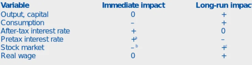
Table 1 summarizes our principal findings. The first column of the table shows the imme-diate impact that the adoption of a consumption tax can be expected to have on each of several variables. The second column shows the long-run impact of tax reform. Ordinarily, when we tax a good or activity, we expect to see less of it in the marketplace. However, a tax on con-sumption causes the economy to achieve a
higher level of consumption, in the long run, than would be observed under an income tax. The resolution of this paradox is that society accumulates greater real wealth under a con-sumption tax than it does under an income tax — an accumulation that is made possible because the initial effect of the consumption tax is to reduce consumption.
Is the eventual increase in consumption worth the initial decline? In the simple model economy examined here, the answer is unam-biguously yes. Because the supply of labor is fixed in our model economy, the only compo-nent of the income tax that is distortionary is the profits tax: it reduces the demand for capital at any given after-tax interest rate. Because the consumption tax eliminates this distortion, it necessarily raises social welfare.
The real world is obviously more com-plicated than our model economy. Most per-tinently, household labor supply is not exogenously fixed: any tax on labor income distorts households’ labor – leisure choices. If moving from an income tax to a consumption tax significantly worsens this labor-market dis-tortion, it may reduce social welfare despite the fact that, at the same time, it eliminates an investment-saving distortion.
Fortunately, it is relatively easy to explain how the results obtained here would change, qualitatively, if the supply of labor was endoge-nous. We address this issue in Part 2 of our article. Part 2 also considers the sensitivity of our results to capital adjustment costs and to a specification of the production function that has each firm’s output depend on the aggregate
capital stock as well as its own.
NOTES
1 Howitt and Sinn (1989) undertake a more
sophisti-cated analysis within a similar framework.
2 For simulation exercises that examine the impact of tax
reform on different age groups, see Auerbach and Kotlikoff (1987) and Auerbach (1996). Feenberg, Mitrusi, and Poterba (1997) present a careful analysis of the impact of tax reform on the distribution of consumption.
Sarkar and Zodrow (1993) discuss windfall gains and losses resulting from tax reform and how they might be mitigated. Monetary policy affects the distribution of wealth primarily through unanticipated inflations, which benefit debtors at the expense of lenders, and unan-ticipated deflations, which have the opposite effect.
3
Hines (1996) contains a general discussion of compli-cations that arise in an open-economy setting. Mendoza and Tesar (1995) construct a formal model.
4
In otherwise identical models, the inclusion of a pre-cautionary savings motive cuts the impact of tax reform on output, consumption, and the capital stock roughly in half.
5
According to the Federal Reserve Board’s flow of funds accounts for the nonfarm, nonfinancial corporate business sector, internal funds averaged 94.8 percent of capital expenditures over the ten-year period from 1985 through 1994. In contrast, credit market borrow-ing averaged only 32.5 percent of capital expenditures.
6
For more detailed descriptions of these alternative approaches, see Koenig and Taylor (1996), Hall and Rabushka (1996), Metcalf (1996), and Moore (1996).
7
We ignore human capital and the associated invest-ment in education and training.
8
The statutory tax rate on corporate profits is 35 per-cent. The tax rate on wage income can be obtained by adding 14 percent (representing federal payroll taxes) to the 22 percent marginal income tax rate reported in Auerbach (1996). The actual tax rates on household interest and dividend income are 22 percent and 27 percent, respectively (Auerbach 1996). For compari-son, Mendoza, Razin, and Tesar (1994) obtain an esti-mate of 32 percent for the U.S. corporate capital income tax rate and an estimate of 34 percent for the tax rate on U.S. labor income. Triest (1996) estimates a 38 percent average marginal tax rate on labor income. Personal income tax deductions and exemptions that are excluded from our model (and that would be elimi-nated under most tax-reform proposals) account for the relatively low revenue yield of the current system, despite high marginal tax rates.
9
Triest’s (1996) estimate of the required flat-tax rate (39 percent) is somewhat higher than ours, but not much different from his own estimate of the current average marginal tax rate on labor income (38 percent).
10
The alert reader will have noted that the transition can
Table 1
Impact of Fundamental Tax Reform in the Basic Model
Variable Immediate impact Long-run impact
Output, capital 0 +
Consumption – +
After-tax interest rate + 0
Pretax interest rate +a –
Stock market –b +c
Real wage 0 +
NOTES:a
Assumes that profits are currently taxed more heavily than is interest.
b Assumes that the new tax rate on corporate cash flow will exceed the current tax rate
on dividends.
c Assumes that (1 – τ)k
be completed in a single step by setting τp= 0 and τw = τd ≡ τ ′. However, this approach breaks down in the real world, where not every firm is able to finance its capital investment out of its own retained earnings.
11
If 1 + rt> MRS (ct, ct + 1), then it will be advantageous
to the household to reduce its period-t consumption by one unit and buy a bond. Principal and interest on the bond (received in period t + 1) will be more than enough to compensate the household for the reduction in ct. Similarly, if 1 + rt< MRS (ct, ct + 1), then it will be
advantageous to the household to sell a bond from its portfolio and use the proceeds to increase its period-t consumption by one unit.
12 These estimates are meant to convey no more than the
likely order of magnitude of the economy’s response to tax reform. They are sensitive to the assumed profits tax rate and to the assumed capital-elasticity of output. Other studies have generally reported a slightly weaker baseline output response.
13 Moreover, we implicitly switch to a continuous-time
version of the model described above.
14 Think of a marble on a saddle. The surface of the
sad-dle looks like a U when viewed from the side and like an inverted U when viewed from either end. The point in the middle of the saddle is the steady state. A mar-ble placed precisely at this point will remain stationary. In principle, a marble placed at the exact middle of one of the saddle’s ends will move toward the steady state rather than fall off the saddle on either side.
15 For a gradual reform analysis, see Howitt and Sinn (1989).
REFERENCES
Auerbach, Alan J. (1996), “Tax Reform, Capital Alloca-tion, Efficiency, and Growth,” in Economic Effects of Fundamental Tax Reform, eds. Henry J. Aaron and William G. Gale (Washington, D.C.: Brookings Institution Press), 29 – 82.
Auerbach, Alan J., and Laurence J. Kotlikoff (1987), Dynamic Fiscal Policy (Cambridge, England: Cambridge University Press).
Engen, Eric M., and William G. Gale (1997), “Consump-tion Taxes and Saving: The Role of Uncertainty in Tax Reform,” American Economic Review Papers and Proceedings 87 (May): 114 –19.
Engen, Eric M., Jane Gravelle, and Kent Smetters (1997), “Dynamic Tax Models: Why They Do the Things They Do,” National Tax Journal 50 (September): 657– 82. Feenberg, Daniel R., Andrew W. Mitrusi, and James M. Po-terba (1997), “Distributional Effects of Adopting a National Retail Sales Tax,” inTax Policy and the Economy, ed. James M. Poterba (Cambridge, Mass.: MIT Press), 49 – 89. Gentry, William M., and R. Glenn Hubbard (1997),
“Distributional Implications of Introducing a Broad-Based Consumption Tax,” in Tax Policy and the Economy, ed. James M. Poterba (Cambridge, Mass.: MIT Press), 1– 47. Hall, Robert E., and Alvin Rabushka (1996), “The Flat Tax: A Simple, Progressive Consumption Tax,” in Frontiers of Tax Reform, ed. Michael J. Boskin (Stanford, CA: Hoover Institution Press), 27– 53.
Hines, James R. (1996), “Fundamental Tax Reform in an International Setting,” in Economic Effects of Fundamental Tax Reform, eds. Henry J. Aaron and William G. Gale (Washington, D.C.: Brookings Institution Press), 465 – 502. Howitt, Peter, and Hans-Werner Sinn (1989), “Gradual Reforms of Capital Income Taxation,” American Economic Review 79 (March): 106 – 24.
Koenig, Evan F., and Lori L. Taylor (1996), “Tax Reform: Is the Time Right for a New Approach?” Federal Reserve Bank of Dallas Southwest Economy, Issue 1, January/ February, 5 – 8.
Mendoza, Enrique G., and Linda L. Tesar (1995),“Supply-Side Economics in a Global Economy,” International Finance Discussion Paper no. 507 (Washington, D.C.: Board of Governors of the Federal Reserve System, March). Mendoza, Enrique G., Assaf Razin, and Linda L. Tesar (1994), “Effective Tax Rates in Macroeconomics: Cross-Country Estimates of Tax Rates on Factor Incomes and Consumption,” Journal of Monetary Economics 34 (December): 297– 323.
Metcalf, Gilbert E. (1996),“The Role of a Value-Added Tax in Fundamental Tax Reform,” in Frontiers of Tax Reform, ed. Michael J. Boskin (Stanford, CA: Hoover Institution Press), 91–109.
Moore, Stephen (1996),“The Economic and Civil Liber-ties Case for a National Sales Tax,” in Frontiers of Tax Reform, ed. Michael J. Boskin (Stanford, CA: Hoover Institution Press), 110 – 20.
Sarkar, Shounak, and George R. Zodrow (1993), “Transi-tional Issues in Moving to a Direct Consumption Tax,” National Tax Journal 46 (September): 359 – 76.
Slemrod, Joel (1996), “Which Is the Simplest Tax System of Them All?” in Economic Effects of Fundamental Tax Reform, eds. Henry J. Aaron and William G. Gale (Washington, D.C.: Brookings Institution Press), 355 – 91. Triest, Robert K. (1996), “Fundamental Tax Reform and Labor Supply,” in Economic Effects of Fundamental Tax Reform, eds. Henry J. Aaron and William G. Gale (Washington, D.C.: Brookings Institution Press), 247–78.
It will be useful to consider an example of an economy as described in the main text, which will enable us to quantify the responses to fundamental tax reform. Consider an environment in which households are identical and have preferences described by a utility function of the form
∑∞t = 1log(ct)/(1 + ρ)t,
where ctis household consumption at timet, and ρ is the pure rate of time preference. With this utility function, the marginal rate of substitution between current and future consumption [MRS (ct, ct + 1)] is simply (1 + ρ)(ct + 1/ct ). Consistent with Equation 3, the optimality condition 1 + rt= MRS (ct, ct + 1) takes the form
where rtis the real after-tax interest rate. We assume that production per household is a simple function of capital per household:y = kθ. It follows that the marginal product of capital (MPk) is θkθ– 1. Investment optimality conditions (Equa-tions 5 and 5′for an economy with an income tax and an economy with a consumption tax, respec-tively) become
rt= (1 – τp)(θktθ– 1
– δ) and
rt= θktθ– 1– δ,
where δis the depreciation rate for capital and τpis the corporate income tax rate. Finally, Equation 7, which governs the evolution of the capital stock, takes the form
kt + 1– kt= ktθ– ct– gt– δkt,
where gtdenotes government purchases at timet. We assume that a period is a quarter of a year and let ρ= 0.01 and δ= 0.02. These parame-ter values imply that the average annual rate of return on capital is just over 4 percent in steady state, and the annualized depreciation rate is just over 8 percent. The technology parameter, θ, is set equal to 0.35. Government purchases are constant through time.
Figures A, B, and C show the response of the capital stock, consumption, and after-tax rate of return to fundamental tax reform. Initially, the economy is assumed to be in steady state with a corporate income tax rate of 35 percent. (Interest, dividend, and wage taxes may also be in effect, but these are irrelevant to our simulations.) Suddenly, in period 0, the income tax is replaced by a con-sumption tax. In the figures, the initial steady-state levels of consumption and capital are normalized to unity. As can be seen, convergence is fairly com-plete after 100 periods, or 25 years. However, con-sumption does not rise above its initial steady-state level for 40 periods, or 10 years. The after-tax annual interest rate jumps from 4.1 percent to around 6.3 percent before gradually falling back to its old level. As noted in the main text, the pretax interest rate (not shown in the figures) may jump upward or downward when tax reform is imple-mented, depending upon the relative magnitudes of the tax rates on interest income and corporate
c c r t t t + = + + 1 1 1 ρ,
A NUMERICAL EXAMPLE
profits. Assuming that interest income is initially taxed at a 25 percent annual rate, tax reform would see the pretax interest rate jump upward from 5.4 percent to 6.3 percent, then gradually fall to 4.1 percent.
Figure A
Capital
Index, initial steady state = 1
.90 .95 1 1.05 1.10 1.15 1.20 1.25 1.30 Time (quarters) 100 50 0 Figure C
After-Tax Interest Rate Percent per year
4 6.5 6 5.5 5 4.5 Time (quarters) 100 50 0 Figure B Consumption Index, initial steady state = 1
.80 1.05 1 .95 .90 .85 Time (quarters) 100 50 0