Worcester Polytechnic Institute
Digital WPI
Masters Theses (All Theses, All Years) Electronic Theses and Dissertations
2013-12-23
Scalable Multi-Parameter Outlier Detection
Technology
Jiayuan Wang
Worcester Polytechnic Institute
Follow this and additional works at:https://digitalcommons.wpi.edu/etd-theses
This thesis is brought to you for free and open access byDigital WPI. It has been accepted for inclusion in Masters Theses (All Theses, All Years) by an
authorized administrator of Digital WPI. For more information, please [email protected].
Repository Citation
Wang, Jiayuan, "Scalable Multi-Parameter Outlier Detection Technology" (2013).Masters Theses (All Theses, All Years). 1147.
Scalable Multi-Parameter Outlier Detection Technology
by Jiayuan Wang
A Thesis
Submitted to the Faculty of the
WORCESTER POLYTECHNIC INSTITUTE In partial fulfillment of the requirements for the
Degree of Master of Science in
Computer Science by
Jan 2014
APPROVED:
Professor Elke A. Rundensteiner, Thesis Advisor
Professor Mohamed Eltabakh, Thesis Reader
Abstract
The real-time detection of anomalous phenomena on streaming data has become increas-ingly important for applications ranging from fraud detection, financial analysis to traffic management. In these streaming applications, often a large number of similar continuous outlier detection queries are executed concurrently. In the light of the high algorithmic complexity of detecting and maintaining outlier patterns for different parameter settings independently, we propose a shared execution methodology called SOP that handles a large batch of requests with diverse pattern configurations.
First, our systematic analysis reveals opportunities for maximum resource sharing by leveraging commonalities among outlier detection queries. For that, we introduce a sharing strategy that integrates all computation results into one compact data structure. It leverages temporal relationships among stream data points to prioritize the probing process. Second, this work is the first to consider predicate constraints in the outlier detection context. By distinguishing between target and scope constraints, customized fragment sharing and block selection strategies can be effectively applied to maximize the efficiency of system resource utilization. Our experimental studies utilizing real stream data demonstrate that our approach performs 3 orders of magnitude faster than the start-of-the-art and scales to 1000s of queries.
Acknowledgements
I would like to express my gratitude to my advisor professor Elke Rundensteiner. Thank for her continuous support for my research and thesis work. Thank for her time on revising my thesis again and again, to make it perfect. I really appreciate her patient guide, encouragement, as well as immense knowledge, which help me to continuously grow and improve during my master study.
My thanks also go to my thesis reader professor Mohamed Eltabakh, for his valuable advises on my thesis work, which helps me to improve the quality of this thesis.
I also thank the mentor in WPI DSRG: Lei Cao, for all the inspirations and feedbacks on my research work.
I thank all my DSRG member in WPI: Chuan Lei, Xizhao Chen, Di Yang, Medhabi Ray, Xika Lin, Qingyang Wang for all the feedbacks and discussion on my work;
Lastly, I want to thank my whole family: my parents Zhihe Wang and Xiaoying Chen. Thank for giving me tremendous support for no matter my life or study.
Contents
1 Introduction 1
1.1 Motivation . . . 1
1.2 State-of-art Limitations . . . 3
1.3 Challenges & Proposed Solution . . . 4
1.4 Contributions . . . 6
2 Distanced-Based Outlier Detection Basics 8 2.1 Basic Concepts . . . 8
2.2 Outliers in Sliding Windows . . . 9
3 Problem Formalization 12 3.1 A General Problem . . . 12
3.2 A Running Example . . . 14
4 Sharing Among Queries with Pattern and Window Parameters 15 4.1 Varying Parameter - K . . . 15
4.2 Varying Parameter - R . . . 19
4.3 Varying Parameter - K and R . . . 23
4.4 Varying Parameter - W . . . 25
4.6 Varying Parameter - W and S . . . 30
4.7 Varying Parameter - K, R, W and S . . . 32
4.8 Complexity Analysis . . . 32
5 Sharing Among Queries with Predicate Parameters 35 5.1 Intuitions and Approaches . . . 37
5.2 Complexity Analysis . . . 43
6 Performance Evaluation 44 6.1 Experiment Setup and Methodology . . . 44
6.2 Evaluation of SOP for Varying Pattern and Window Parameters . . . 46
6.2.1 Varying Pattern-Specific Parameters . . . 46
6.2.2 Varying Window-Specific Parameters . . . 51
6.2.3 Varying Pattern and Window Specific Parameters . . . 54
6.3 Evaluation of SOP For Varying Predicates . . . 55
6.3.1 Varying Target Sharing Percentage . . . 55
6.3.2 Varying Scope Sharing Percentage . . . 57
6.3.3 Scalability on Predicates . . . 57
7 Related Work 59
8 Conclusion 63
List of Figures
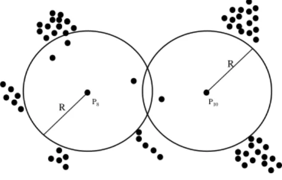
2.1 An example data set with two distance-based outliers . . . 9
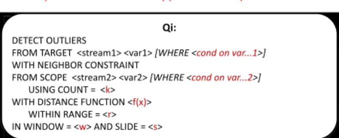
3.1 Query Template . . . 14
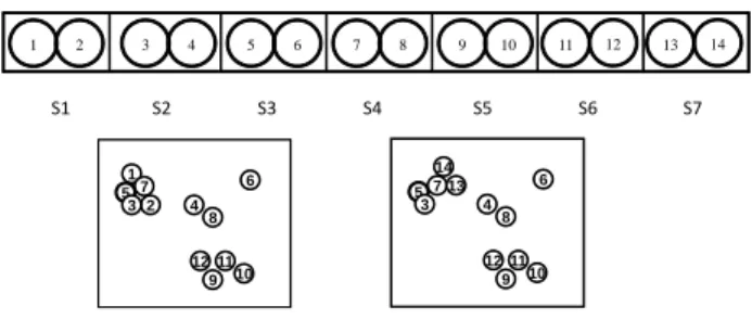
4.1 Distribution of data points . . . 18
4.2 Arbitrary K: neighbor information . . . 19
4.3 Arbitrary R: neighbor information . . . 22
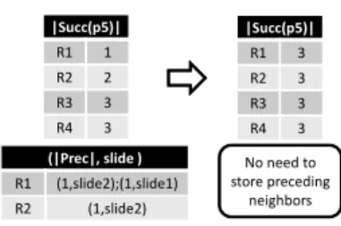
4.4 Matching table . . . 25
4.5 Arbitrary W: neighbor information . . . 29
5.1 Geographic Distribution and Window View . . . 36
5.2 Unshared Predicates . . . 36
5.3 Possible Fragments . . . 38
5.4 Conceptual View of Fragments Sharing . . . 39
5.5 Possible Blocks in Two Different Case . . . 40
6.1 Varying K values on Synthetic Dataset . . . 47
6.2 Varying R values on Synthetic Dataset . . . 49
6.3 Varying K and R values on Synthetic Dataset . . . 50
6.4 Varying W values on Synthetic Dataset . . . 51
6.5 Varying S values on Synthetic Dataset . . . 53
6.7 Varying K, R, W and S values on Synthetic Dataset . . . 54
6.8 Varying Predicate Sharing Percentage on Synthetic Dataset . . . 56
List of Tables
6.1 Parameters Setting of SOP . . . 46
Chapter 1
Introduction
1.1
Motivation
Nowadays, almost all information is generated, transmitted, and stored as digital data, giving rise to a prevalent focus on how to extract insight from those huge volumes of data. Outlier detection [8] is one popular technique to identify anomalous patterns and then interpret them as the phenomenon in the real world. We can catch a glimpse of its increasing importance in many modern applications in a variety of fields ranging from fraud detection, traffic management, damage evaluation to economical analysis.
The idea of detecting outliers originates from the notion of capturing abnormal phe-nomena in data put forward in [21]. An abnormal phenomenon is introduced as the core principle that outliers can be identified by using the similarity among points in a dataset. Based on this foundation, one important class of distance-based outlier definitions stands out [5,8,22,23]. The one we used in this paper is given initially in [5] where outlier is an object O with fewer than k neighbors in the database, where a neighbor is an object that is within a distance R from object O. This definition fits well for applications where the threshold for outlier is clear.
In many applications a popular data stream is monitored by many analysts [12,13,14,15,16]. For example, some financial analysts may continuously monitor the stock transaction streams from the New York Stock Exchange to evaluate their stability. They might detect a widely-fluctuating real estate stock by bounding the range of the purchasing price differ-ence from 100 to 200USD and set the configurations for number of neighbors needed at 30 for similar transactions. Meanwhile, other analysts might prefer to use a more relaxed demarcation line to delineate unstable performance, setting the range from 80 to 220USD or the number of similar transactions to 20. Also, some may be interested in the stability across one year, while others may submit queries with a much shorter time span such as six months. Thus applications may receive a huge workload of similar concurrent queries with different pattern-specific and window-specific parameter settings over the same data stream. Accordingly some strategies should be applied to process this workload of simi-lar outlier detection queries to serve applications in real time, by reducing the processing time and increasing the efficiency of delivery of results.
Most optimization principles on sharing system resources are concentrated on pattern-specific and window-pattern-specific parameters [7]. To date, predicates have not yet been consid-ered in the outlier detection context. Yet predicates are crucial in expressing the semantics of outliers. For instance, the stocks that some analysts are interested in are confined to Boston only, while others might pay attention to stocks to watch the economy in Mas-sachusetts. Moreover, sometimes whether a data point is an outlier does not entirely rely on the condition of the stream it belongs to. Rather it is common that several data streams need to be considered in context. Again, considering the stock example, the stability of real estate stocks in Boston may be relevant to the stability of building material stocks in Massachusetts, or even the larger scope of material stocks under the USA. Therefore, assuming real estate stocks in Boston are the original streams then building material s-tocks are streams we use to compare against. Predicates play a role to control and filter
these streams. Clearly, a system that supports hundreds of outlier detection queries with predicates is extremely resource intensive.
1.2
State-of-art Limitations
Handling a huge workload of different outlier detection queries on a single system con-tinuously under high input rates is a challenging problem. Accordingly, although the state-of-the-art method [1] that efficiently deals with a single distance-based outlier de-tection query has been proved to be optimal theoretically, executing each of the queries independently via using this method still has prohibitively high demands on both com-putational and memory resources. For example, it takes LEOC [1] 10s to update the processing query results with 1M data points in the window, then it would take us 1000s to process 100 queries by executing LEOC 100 times. This does not meet the real time responsiveness requirement and thus would be prohibitively costly. Thus the method on a single query is not feasible and applicable for practical applications, especially when the number of queries to be executed is large. Therefore, we now propose to leverage the insights and technique of LEOC while designing a resource-shared query processing approach to process a huge of workload of queries.
With regards to lots of extensively researched solutions on the shared workload of outlier detection queries processing [2,4], they reduce the massive system resource uti-lization caused by the full scan of the whole window for each points being processed. One of the cutting-edge approaches proposed in [2] scales to handle a large quantity of queries where only pattern-specific parameters, namely number of neighbors K and neigh-bor search range R, are supplied. More specifically, they do not take the window-specific parameters into consideration. Also, they do not support predicates. In addition, the main idea of its outlier detection is based on the single query strategy [2], which is based on
the expensive range query during the search process.
Predicates are known to play an important role in screening the data we are interested in by signifying selection conditions in a query. However, none of the existing outlier techniques [1,2,6] integrates predicates as parameters into the outlier detection process. One insightful sharing strategy [3] of predicates in streaming data environments comes up with an idea of dividing the data set into fragments with different signatures attached to recognize lists of queries that they belong to. We leverage their method to maximize the resource sharing of arbitrary selection predicates. However, prior work concentrates on aggregation only, it is not possible to directly be applied to outlier detection query processing. Especially in our case where the evaluation of the outlier qualification of data points in one stream sometimes depends on another data stream. This implies that outlier detection can involve several data streams instead of a particular one in tradition. The one to be detected and the one to be probed. Based on this idea, predicates can be put on both.
1.3
Challenges & Proposed Solution
This paper is to design, implement and evaluate an optimized technique for processing multiple outlier detection queries in streaming environments. The efficient algorithm we propose, called SOP, handles a huge workload of queries varying three parameter sets where each two variations are contained. They include the number of neighbors K, search range R, window size W, sliding size S, predicate TARGET and predicate SCOPE respectively. In our framework, we introduce several innovative strategies and search operations for optimizing the shared processing of multiple queries to ease the burden of available CPU and memory resources.
First, we design the status indicator technique that takes advantage of the relationship between the parameter setting values in different but similar outlier detection queries. For
queries with less restricted specifications on parameter settings, their outputs are com-pletely contained in the results of queries with more restricted parameter settings. Based on this observation, namely pattern containment, using the status indicator allows us to handle multiple queries without maintaining separate details about a workload of queries. Then we propose a technique so that we simply keep least evidence sufficient for the most restricted queries instead of routinely conducting expensive range queries to gain all qualified neighbors.
Second, we also present a technique to handle predicate parameters in our distance-based outlier detection process. In light of the demands from the real world request, outliers to be detected sometimes are not only being confirmed as abnormal from data streaming they belong to. Instead, their identification of the outlier status depends on some other related data streams. Therefore data streams can be categorized into target and scope based on their purpose in outlier detection queries. Target is the stream where data reside to be evaluated if they are outliers or not and scope is the stream that all target data probe into to find neighbors. By dividing target data into fragments and scope data into blocks based on different predicates specifications on target and scope, we do not have to use brute force to apply our outlier detection technology on data stream over and over. We aim to utilize the uniqueness of fragments and blocks to actualize sharing purpose when executing outlier detection technology. This is based on the characteristic that all data contained in one fragment or block will not be included in other fragments or blocks at the beginning when they are established. Meanwhile we exploit the bitmap as a signature to signify different fragments and blocks we are detecting and probing as well as the lists of associated queries, keeping track of the outputs for each query. Thus duplicate computations can be avoided.
Lastly, our experimental studies on both synthetic and real data demonstrate that SOP successfully reduces the CPU and memory utilization significantly by almost three
or-ders of magnitudes, confirming the effectiveness and superiority over the state-of-the-art alternatives.
1.4
Contributions
In our SOP approach, we successfully tackle all problem outlined above. Contributions of our work on solving this real time outlier detections of multiple queries are summarized as follows:
1) We introduce the concept of a status indicator to efficiently share same patterns for different outlier detection queries. This frees the repeatedly executions on the same data stream which is common for the state-of-the-art methodology [1].
2) We present the least search technique that plays a role in controlling the timing of neighbor search termination. The appropriate termination can minimize the number of comparisons before sufficient evidence for a data point is collected without neglecting to compare some other data points when delivering outliers for all queries in the workload.
3) We integrate these techniques into one framework to enable general parameter set-tings on outlier detection in streaming environments.
4) We propose an innovative way to incorporate predicate parameters into outlier de-tection specification settings by fragment sharing strategy and block selection operation on Target and Scope separately to share overlapped portions in predicates. No other ap-proach of sharing of outlier detection is known to support this rich set of parameters.
5) We validate the improved performance of our approach with experiments against other edge-cutting methods on both synthetic and real data.
The rest of the paper is organized as follows. Chpater 2 briefly introduces the pre-liminary knowledge about distance-based outlier detection and the problem formalized in 3. The technique of SOP on sharing strategies given multi-query with arbitrary parameter
settings is given in Chapter 4 and Chapter 5. Experimental results are analyzed in Chapter 6. Chapter 7 covers related work, while Chapter 8 concludes the whole paper.
Chapter 2
Distanced-Based Outlier Detection
Basics
2.1
Basic Concepts
Outliers generally is described as objects that behave differently from the ”typical case”. In recently years, several outlier definitions have been developed to separate outliers from the normal majority. One of the most widely used definitions is based on distance [2,3]: if there are less than k objects within a distance of range r for an object A, then A is considered as an outlier. We use the following definition of distanced-based outlier to
define outliers. The function dist (pi, pj) is used to denote the distance between data
pointspiandpj. Given the distance threshold R, function nn (pi, R) represents the number
of neighbors a data objectpi has within range R.
Definition 1: Given R and parameter k (k¿0), if nn (pi, R) ¡ k, thenpi is regarded as
R
R
P8 P10
Figure 2.1: An example data set with two distance-based outliers
2.2
Outliers in Sliding Windows
One distinguishing trait of streaming data compared to static data is its infinity. Another feature is the high velocity when streaming data arrive the system. This high speed and volume arouse the difficulties in maintaining and processing all these on-the-fly data at real time. In order to tackle streaming data, a sliding window semantics that is widely used in literature [6,7] is taken out so that we can chopped infinite streaming data into continuous finite snapshots and then apply our outlier detection algorithm in each snap-shot. With this window mechanism, we are able to overcome the difficulties caused by the huge volume and high arrival speed of data stream.
Meanwhile, it is well known that most analysts are more interested in the fresh data. This is because fresh data always contains more useful information hidden behind. Ac-cordingly, among outlier detection analysis, it is the most recent data that are the main focus instead of the ancient one. Window mechanism is propitious to the processing of newly-arrived data and the expiration of old ones.
However, when applying window mechanism in the distance-based outlier detection, arrival and expiration of data points inevitably affect the total number of neighbors of each data point in the latest window. This is because neighbors change over sliding
win-dow. Hence, capability of dealing with this instability obviously becomes one of the most system-resource-consuming considerations of the query processing tasks.
Here we give an example of how naive distance-based outlier detection in sliding window works. Assume that there is a distance-based outlier detection query with R
specified as 5 and K specified as 3. Data point pi havep1, p3, p7 andp9 as neighbors in
the current windowW1. After 5 seconds, window slides. p1 andp3 expire and no longer
can be counted as the neighbors ofpi. Meanwhile, there are no more neighbors found in
the new-arrived data. At this pointpionly collects two neighbors. Accordingly, we claim
thatpibecomes an outlier after window slides.
In streaming database systems, we assume all arriving data points have their own
unique timestamps, denoted as pi.ts. Ifpi.ts is greater than pj.ts, it means thatpi arrives
earlier thanpj. For all neighbors ofpiwhose timestamp is less thanpi.ts, we signify those
neighbors as preceding neighbors ofpi, denoted as set P(pi). Likewise, all neighbors ofpi
whose timestamp is larger thanpi.ts, we signify those neighbors as succeeding neighbor
ofpi, denoted as set S(pi). For all data points∈S(pi), they can always be considered as
neighbors ofpi no matte how window slides. Only data points∈S(pi) cause the change
of total number of neighbors. In the above case,p1 andp3 are preceding neighbors ofpi
whilep7andp9 are succeeding neighbors ofpi.
This observation gives us an insightful view to classify data point into three different
categories based on the size of S and P. For a data pointpi, if the size of S(pi) ¿= k, thenpi
is a safe inlier. We denoteIsas the set of safe inlier. This meanspiis guaranteed to never
become an outlier at any time. If the size of S(pi) ¡ k, yet the size of P(pi) + S(pi) ¿= k,
thenpiis an unsafe inlier.Iuis used to denote the set of unsafe inlier. This indicates when
some neighbors in P(pi) expire, pi has a chance to become an outlier ifpi is not able to
find more neighbors in newly-arrived data point. Otherwise, if the number of data points
Chapter 3
Problem Formalization
3.1
A General Problem
Generally, when an analyst is not certain about the best parameter settings for his analysis, he might submit multiple queries of the same type but with different parameter settings at the same time. Moreover, the data streaming he has been concentrating on is entirely possible being monitored by other analysts simultaneously. Therefore, efficiently sharing among computation results from both intermediate and output ones multiple of outlier detection queries that have arbitrary pattern-specific and window-specific parameters is our goal. To actualize it, the main problem we need to settle is how to share and maintain the progressive pattern in the real-time responsiveness applications.
Here is a general description of multiple queries with arbitrary pattern-specific and window-specific parameters. Given a workload of WL with n distance-based outlier
de-tection queriesQ1(S,k1,
r1,w1,s1), Q2(S,k2,r2,w2,s2), ...,Qn(S,kn,rn,wn,sn) querying the same input data stream
S, while all the other query parameters such as k, r, w and s differ.
out-liers they are trying to find with the data stream where outout-liers reside only. However, under many conditions, it is entirely possible for outliers and their neighbors coming from totally distinct multiple data streams. Therefore we categorize data stream into two types based on the demands of analysis purposes. Data stream in which all data points are the ones we would like to evaluate whether they are outliers or not is Target stream. Data stream that we probe into to see whether data points in it are neighbors of the data points in Target stream or not is Scope stream. Based on the definition of distance based outlier, Target and Scope streams can be irrelevant because what to analyze and what to probe can be totally different.
In addition, so far none of the known outlier detection technologies have been devel-oped to support predicates sharing. However, providing another predicate type param-eters, which is not the common case in outlier detection, serves to be extremely useful in practical applications. Accordingly, besides two pattern specific and window specific parameters, we aim to integrate two predicates parameters into our outlier detection algo-rithm dealing with multiple queries. Based on the type of data stream they are applying to, they are Target predicate and Scope predicate. It is Target predicate if the filter is put on the Target stream. Otherwise if filter is put on the Scope stream, then this predicate is Scope predicate. Again, in order to share the computations and results of the progres-sive pattern, it is crucial to exploit the similarities among those predicates specified by different queries to improve performance efficiency.
Figure 3.1 is the query template with the predicate parameters extended from the gen-eral outlier query template [7]. In this complete query template, the gengen-eral formulation of a query with arbitrary predicate parameters as well as pattern-specific and window-specific parameters is fully illustrated. What need to be paid attention to is that Scope stream is not only restricted to simply one data stream. Disparate Scope streams can be pulled together through union operation into this template.
• Input: a query group QGwith multiple outlier-detection queries on
some input streamswith arbitrary predicates and parameters.
• Goal: to minimize both the average processing time and the memory space needed by the system.
Template Outlier Detection Query Over Sliding Windows Qi:
DETECT OUTLIERS
FROM TARGET <stream1> <var1> [WHERE <cond on var...1>]
WITH NEIGHBOR CONSTRAINT
FROM SCOPE <stream2> <var2> [WHERE <cond on var...2>]
USING COUNT = <k> WITH DISTANCE FUNCTION <f(x)>
WITHIN RANGE = <r> IN WINDOW = <w> AND SLIDE = <s>
Figure 3.1: Query Template
3.2
A Running Example
Here we introduce a concrete example of how an outlier query with predicates can be formalized in the query template. The main purpose of the query is to detect users in HR Dept who behaves strangely in the latest hour and keep updating every one minute. The definition of strange behavior, in this query, is bound by the fact that their login or access times on 10 different machines or 10 different files should be more than 30 times.
From description above. Target stream is users. Scope stream is different machine login files and file access files. K is 30 times. R is 1o files. W is 60 minutes. S is 1 minute. Both target and scope predicate are HR Dept.
Chapter 4
Sharing Among Queries with Pattern
and Window Parameters
We now propose our approach in optimizing the process of a workload of queries with arbitrary pattern-specific and window-specific parameters. Our sharing outlier process-ing (SOP) algorithm mainly is based on the minimization of neighbor search times, the maintenance of progressive pattern over sliding window among multiple queries and shar-ing on both intermediate and output results. By applyshar-ing these strategies durshar-ing outlier detection execution process, SOP can continuously generate an evolving result set and provide answers to queries with all possible combinations of different-pattern specific and window-specific parameters.
4.1
Varying Parameter - K
Consider the window-specific parameters and one of the pattern-specific parameters R are the same for the workload of many queries with different K values. This implies that all queries share the window size, slide size, range and require output at the same time, while
outlier data points that need to be reported for each query differ.
Assume that queries in the workload are ascendingly ordered in the light of the value of K from min to max. The total neighbor number of each data point in the workload is a constant number after the neighbor search stops. It has nothing related with different K values among queries. Based on this observation, we can infer that under the situation where only K is the variable parameter, we just need to maintain the number of neighbors equivalent to the largest K value. Once the largest K neighbors have been found, then it is sufficient to answer all the queries lined up whose K values are less. In this way, full share is thus achieved.
Status Sharing Lemma: Given a workload WL of queries with arbitrary K
param-eter setting. After neighbor search stops, if data point pi ∈ Is for queries with K
val-ue ki (0¡i¡number of different k,kmin¡ki¡=kmax) in WL, then safe status indicator of pi
will be indexed as ki. If pi ∈Iu for queries with K value kj (0¡j¡number of different k, kmin¡kj¡=kmax) in WL, then unsafe status indicator ofpiwill be indexed askj. For those
queries whose K valuekk¿kj,pi ∈D.
Proof: This Lemma holds because in arbitrary K case, there is an inclusion
relation-ship based on the number of neighbors for ascendingly ordered arbitrary K queries. This pattern containment relationship enables the sharing by using a status indicator. Status in-dicator just records two indexes referring to threshold based on the value of K, safe status
indexIsand unsafe status indexIu. As long as certain number of succeeding neighbors,
sayki, ofpi is maintained, thenpi is a safe inlier to queries whose K values are less than
ki. Therefore by setting up the safe status index atki, we are able to indicate the threshold
that to which queries this data point is safe inlier and to which not. Otherwise, if less
thankj neighbors are collected, then based on the pattern containment relationship, status
indicator can be used to at least show the divide of which queries can report this data point
all queries whose K values are greater than Iu, pi would be outputted as an outlier, the
rest of the queries in the workload will not.
Following this lemma, we just need to try to find enough neighbors for the query with greatest K value. This simplifies the multi-query sharing problem into single query problem. The only difference is for multi-query sharing, status indicator is additionally maintained. This leads to an important fact which is when to determine the termination of neighbor searching. This can be a quite decisive factor in saving system resources. This is so because if neighbor searching terminates too early, it is entirely possible that
pi can not find enough neighbors due to not touching every data point in the window.
Error output might be caused by such early termination. On the contrary, if we keep searching neighbors even enough neighbors are collected, then redundant comparisons are wasting many precious resources. So late termination of neighbor searching also cause inefficiency. Therefore an inappropriate cutoff time actually significantly influences the efficiency of sharing strategy. Here we give the definition of our Least Search operation for arbitrary K case.
Definition: Given a workload WL with arbitrary K, for each data point pi, Least
Search is the search that first search succeeding neighbors and then preceding neighbors. It will not stop searching neighbors until enough number of neighbors namely greater than or equal to kmax = max{k: for all k specified by queries in WL} within range R
are found. Eventually, if it is unable to find kmax neighbors after all the data points in
alive window have been compared with pi already, then it terminates neighbor search
automatically.
The reason why SOP can use Least Search to exactly ensure the perfect intercept time is because when we are searching neighbors to collect minimum evidence [1] required,
theoretically there are only two situations exist. One is thatpi have found enough
case, thosekmax neighbors are shared by the whole workload, therefore status indicator
ofpi will show thatpi is an inlier for all queries. Continuation of neighbor search would
be unnecessary. Another situation is thatpi cannot findkmax neighbors. In this case, we
could use the status indicator to evaluate to which queries pi is an outlier and to which
ones pi is not. In this way, neighbor search is forcefully terminated because neighbor
search has probed all other data points in the window already.
Example 1Given four queriesQ1, Q2,Q3, Q4 with corresponding K values of 1, 2,
3, 4. R is 1, W is 6 and S is 1. We mainly analyze data point p5. Figure 4.1 shows the
distribution of all data points in the dataset from a distance-based perspective before and after window slides as well as all data points in the current window from a timestamp perspective. 1 2 5 4 3 6 7 8 9 10 11 12 5 4 3 6 7 8 9 10 11 12 13 14 S1 S2 S3 S4 S5 S6 S7 1 2 3 4 5 6 7 8 9 10 11 12 13 14
Figure 4.1: Distribution of data points
Before window slides,p7 is the only succeeding neighbor of p5, therefore —S(p5)—
is updated to 1 indicating the number of succeeding neighbors. Then neighbor search
continues,p1,p2andp3are found as preceding neighbors ofp5, therefore —P(p5, s2)— is
stored indicating there is a neighbor in the second slide and —P(p5, s1)— is maintained
indicating there are two neighbors in the first slide. At this moment, the search stops because the total number of neighbors satisfies 4, the greatest K value. This means it
obtains sufficient evidence, which therefore makes p5 exclude itself from the outlier list
forQ4. Accordingly, the safe status indicator is set to 4 showing thatp5is safe for all four
After window slides,p13and p14arrive as new data points. p1 andp2 are no longer
counted as neighbors of p5 due to the expiration of the first slide. Therefore —S(p5)—
updates to 3 and safe status indicator updates to 3, indicating that p5 is a safe inlier for
Q1,Q2 andQ3. Meanwhile, unsafe status indicator is updated to 4, indicating that forQ4
p5 is an unsafe inlier. So againp5 will not be outputted as an outlier for all queries.
The data structures of how we maintain those neighbor information are shown in Figure 4.2. For succeeding neighbors, only a total number is being updated all the time instead of indexes of some specific data points. However for preceding neighbors, in order to support the event-based mechanism [2] to efficiently schedule the checkups of which data points will be triggered as outliers due to window sliding, we maintain neighbor counts based on the unit of each slides. Status indicator is an additional data structure that indicates the output results that to which queries one data point is an outlier and to which is not by updating its safe inlier index and unsafe inlier index.
|Succ(p5)| 1 (|Prec|, slide ) (1,slide2) (2,slide1) |Succ(p5)| 3 No need to store preceding neighbors
Figure 4.2: Arbitrary K: neighbor information
4.2
Varying Parameter - R
Consider the window-specific parameters and one of the pattern-specific parameters K are same for the workload of a bunch of queries with different R values. This indicates that the window size, slide size, count and require output at the same time are shared by all queries, while outlier data points that need to be reported for each query differ.
Assume that queries are descendingly ordered based on their value of R from max to min. Based on the premise that all the window specific parameters are fixed, as explained
in arbitrary K case that number of neighbors holds a inclusion relationship, this contain-ment relationship still contributes to the sharing strategies in arbitrary R case. This means that number of neighbors found in some queries can also be shared by some other queries
Qiin the workload. More specifically, assume that there are two queries in which R value
ri of queryQ1 is less than R valuerj of queryQ2, then all the neighbors of data pointpi
forQ1obviously can also be claimed as neighbors of ppii forQ2. According to this
obser-vation, once enough neighbors is found within the smallest range, then it is sufficient to answer all the other queries with greater range value. Therefore, full sharing is achieved.
Status Sharing Lemma:Given a workload WL of queries with arbitrary R parameter
setting. After neighbor search stops, if data point pi ∈ Is for queries with R value ri
(0¡i¡number of different r, rmin¡ri¡=rmax) in WL, then safe status indicator ofpi will be
indexed asri. Accordingly, if data point∈Iu for queries with R valuerj (0¡j¡number of
different r,rmin¡rj¡=rmax) in WL, then unsafe status indicator ofpiwill be indexed asrj.
For those queries whose R valuerk¿rj,pi ∈D.
Proof: This Lemma holds because in arbitrary R case, the inclusive relationship of
neighbor number still holds as in arbitrary K case. For descendingly ordered arbitrary R queries, this pattern containment relationship enables the sharing strategy in number of neighbors within different range. This means if number of neighbors of one data point
in the most restricted range rmin equivalent to k is maintained, then it is sufficient to
answer the queries with R value greater thanrmin. Otherwise, if less than k neighbors are
collected for the most restricted range, then based on the pattern containment relationship, status indicator can be used to at least show the divide between which queries can report this data point as an outlier and which queries this data point is an unsafe inlier or safe inlier. More specifically, for all queries whose R value is less than or equal to safe status index, data point is safe. For all queries whose R values fall between safe status index and unsafe status index, data point is an unsafe inlier. It has a potential to become an outlier
due to expiration of its preceding neighbors at some point. Otherwise, queries whose R values less than unsafe status index will output data point as an outlier.
However, there is a difference between arbitrary K case and arbitrary R case in sta-tus sharing strategy. For arbitrary K case, neighbor sharing is bidirectional. This means queries with larger K values can share neighbors with queries with smaller K values and vice versa. Yet in arbitrary R case the neighbor sharing is unidirectional. This means only neighbors found by queries with smaller R values can share number of neighbors with queries whose R values are greater. Since the sharing in the opposite way is not appli-cable for arbitrary R case, data structures used in arbitrary K case can not be inherited to arbitrary R case directly. We adapt data structure that only maintains number of suc-ceeding neighbors in a fixed range to a relation that maintains the number of sucsuc-ceeding neighbors in disparate range for different queries. The same adaptation can be made to the data structure that maintains preceding neighbors. So we maintain number of preceding neighbors within disparate range based on the unit of slide. Utilizing this relation, we are able to know how many neighbors we still need to find within some specific range. Also we are able to look up the exact number of succeeding neighbors being shared by certain queries. As for status indicator, it remains the same.
When we utilizing this lemma in our outlier detection process, the same as arbitrary K case, when to determine the exact timing of neighbor search termination is a key factor that significantly influences the sharing strategy efficiency. Below defined the rules of how SOP handles the search termination in arbitrary R.
Definition: Given a workload WL consists of all queries with same window specific
parameters and count K parameter but arbitrary R, it always searches succeeding neigh-bors and preceding neighneigh-bors later. For each data point pi, its neighbor search will not
stop until enough number of neighbors namely greater than or equal to K neighbors with-in rangermin = min{r: for all r specified by queries in WL}are found. Otherwise, after
all data points in alive window have been compared with pi and it is unable to find k
neighbors within range rmin, then neighbor search terminates automatically because so
far all data points have been touched.
The reason why this definition of least search process is optimal for SOP resembles previously explained reason in the arbitrary K case. After neighbor search stops, there are only two possibilities. One possibility is that pi finds k neighbors within the smallest range. Under this condition, those k neighbors are shared by the whole workload, and
the status indicator of pi will show that pi is an inlier for all queries. Another case is
that pi cannot find k neighbors within smallest range. Under this circumstance, all data
points in the window have already been touched therefore the neighbor search terminates automatically.
Example 2Given four queriesQ1,Q2,Q3,Q4 with corresponding R value of 1, 2, 3,
4. K is 3, W is 6 and S is 1. Again, this time we mainly focus onp5. Distribution of data
points is the same as in Example 1 shown in Figure 2.
Before the window slides, the succeeding neighbors of p5 in four disparate ranges
are shown in Figure 4.3. After compared with all succeeding data points, for Q3 andQ4
who share the same neighbors,p5 is a safe inlier and forQ1 andQ2,p5 is still an outlier,
therefore the neighbor search does not terminate. So it turns back to the preceding data.
When it stops, enough neighbors have been collected for Q1. Hence p5 is no longer an
outlier for all queries. Figure 4.3 shows the preceding neighbors information. Afterwards the safe status is updated to 3 and the unsafe indicator 1.
|Succ(p5)| R1 1 R2 2 R3 3 R4 3 (|Prec|, slide ) R1 (1,slide2);(1,slide1) R2 (1,slide2) |Succ(p5)| R1 3 R2 3 R3 3 R4 3 No need to store preceding neighbors
After the window slides,p13 andp14 arrive as new data points. Caused by the
expi-ration of the first slide, p1 and p2 can not be regarded as neighbors to any data point in
the current window. Therefore p5 loses two of its preceding neighbors, which makes it
become an outlier for Q1 and Q2. So it keeps neighbor search until it finds two
neigh-borsp13andp14 within the smallest range. At this moment, four queries in the workload
share the same number of neighbors and p5 is excluded in the outlier list. Then the safe
indicator is updated to 1.
4.3
Varying Parameter - K and R
Now we consider when both pattern-specific parameters change yet window-specific pa-rameters remain the same for all queries in the workload. This means that the window size, slide size and require output at the same time are shared by all queries, while outlier data points that need to be reported for each query differ.
Because the sharing mechanism and least search process of arbitrary K and arbitrary R case use the same sharing idea and the data structure of those two cases are orthog-onal. Therefore we can naturally combine previous two cases to actualize the sharing mechanism and least search process for arbitrary K and R case.
However, just combining those two cases can lead to extreme situation that consumes unnecessary resources. For instance, there is one query specifying K value as 1 and R value as 1 and there is another query specifying K value as 100 and R value as 100. In this case, least search will require to find 100 neighbors within range 1, which is the most restricted condition. This potentially creates an authentic new query with the most restricted parameter specifications. If we evaluate which data points are outliers for this new created query, extra memory and CPU resources are inevitably wasted.
value is maintained. This table analyzes all arbitrary K and R specifications from all the queries at the first place. Then considering different R values as the primary key of table, corresponding greatest K values are then paired up to them. Accordingly, for each entry in the table, namely one R and its greatest K, it can be processed as a single arbitrary K case. For each column, it can be regarded as a single arbitrary R case. Therefore, without generating new non-existed query and exploiting extra resources consumed by that query is achieved.
Below shows the overall pseudo-code of this combination case in Algorithm 1 and 2.
Algorithm 1SOP(pi,D) Arrival
Require: Data pointpi, DatasetD,R//Dis Data points in the current window,Ris a set of different value of R
1: foreach q∈pi.succPointdo
2: for(ri∈R)do
3: if(true ==pi.isNeighbor(q, r)then
4: for(rj¿=ri)do
5: pi.—Succ(pi,rj)— ++;
6: if(pi.—Succ(pi,ri)— ¿=pi.getKmax(ri))then
7: pi.updateStatusIndicator; 8: break; 9: end if 10: end for 11: end if 12: end for 13: end for
14: whilepi.precSlides! =NULL and !pi.isSafedo
15: slide = getSlideWithLargestLifespan(pi.precSlides(D));
16: foreach q∈slidedo 17: for(ri∈R)do
18: if(true ==pi.isNeighbor(q, r)then
19: forrj¿=rido
20: pi.—Prec(pi,rj)— ++;
21: slide.updateTriggeredList(pi);
22: if( (pi.—Prec(pi,rj)— +pi.—Succ(pi,ri)— ¿=pi.getKmax(ri))then
23: break; 24: end if 25: pi.updateTriggeredSlide(slide); 26: pi.updateStatusIndicator; 27: end for 28: end if 29: end for 30: end for 31: end while
We take the previous example to elaborate this algorithm. It establishes a table with two entries in the first place. One entry is R equal to 1 and K equal to 1. Another one is R equal to 100 and K equal to 100. Utilizing this methodology not only prevents the process of query with extremely restricted parameter specifications, but also takes the advantage
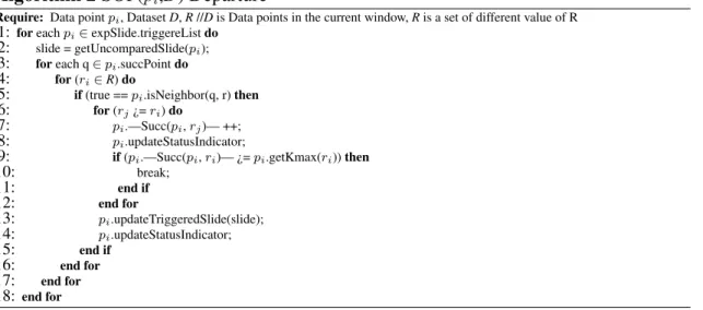
Algorithm 2SOP(pi,D) Departure
Require: Data pointpi, DatasetD,R//Dis Data points in the current window,Ris a set of different value of R
1: foreachpi∈expSlide.triggereListdo
2: slide = getUncomparedSlide(pi);
3: foreach q∈pi.succPointdo
4: for(ri∈R)do
5: if(true ==pi.isNeighbor(q, r)then
6: for(rj¿=ri)do
7: pi.—Succ(pi,rj)— ++;
8: pi.updateStatusIndicator;
9: if(pi.—Succ(pi,ri)— ¿=pi.getKmax(ri))then
10: break; 11: end if 12: end for 13: pi.updateTriggeredSlide(slide); 14: pi.updateStatusIndicator; 15: end if 16: end for 17: end for 18: end for
of sharing strategy and least process to output outliers in real-time response for different queries with less resources being used.
In the line 7 of the Algorithm 1, a data point updates its attached status indicator each time a neighbor is found. Line 14 in Algorithm 1 starts a loop to ensure that neighbor search keeps looking into the fresh data point until enough neighbors has been found.
Figure 4.4 shows another example when the workload consists of four different queries and how the table is established after pre-analyzing.
Query K R a 100 100 b 1 1 c 1 100 d 100 1 R K 1 1, 100 100 1, 100 R K 1 100 100 100
Figure 4.4: Matching table
4.4
Varying Parameter - W
Assuming all the queries start simultaneously, consider the pattern-specific parameters and one of the window-specific parameters S are the same for the workload of a bunch of queries with different W values. This implies that all the queries share the count, range,
slide size and require output at the same time, while outlier data points that need to be reported for each query differ.
Assume that queries are ascendingly ordered based on the value of W from min to max, how to maximize the sharing among queries with different window size now be-comes the main focus. In terms of the definition of streaming system, window of larger size contains the window of smaller size. This means that all slides constituting smaller window are also the slides included in the larger window. The lifetime of data points in the smaller window never terminates in the larger window unless the smaller window slides and no longer keeps them anymore. It is entirely possible that for queries whose
have smaller window sizes thanwmax,piis outputted as an outlier due to no enough
accu-mulating neighbors in all slides contained by those windows. Yet for queries with larger
window sizes or window size being equal to wmax, it is entirely possible that there are
more neighbors of pi residing in other slides, which makespi an inlier for those queries.
Based on this observation, if number of neighbors in each slide contained in the window of larger size is maintained, answering the queries with smaller W value is adequate as well.
Status Sharing Lemma: Given a workload WL of queries with arbitrary W value.
After neighbor search stops, if data pointpi∈Isfor queries with W valuewi(0¡i¡number
of different w,wmin¡wi¡=wmax) in WL, then safe status indicator ofpiwill be indexed as wi. Accordingly, if data pointpi ∈Iufor queries with W valuewj (0¡j¡
number of different w,wmin¡wj¡=wmax) in WL, then unsafe status indicator ofpi will be
indexed aswj. For those queries whose W valuewk¡wj,pi ∈D.
Proof: This Lemma holds because in arbitrary W case, there is an inclusion
rela-tionship among the number of neighbors for ascendingly ordered queries. As long as pattern-specific parameters are same for all queries, then the definition to find outlier is universal in the workload. This means we just need to consider how to chop
progres-sive neighbor numbers into different slides for different window to share. Therefore, we maintain all progressive patterns, especially the number of succeeding neighbors that are used to be maintained based on unit of window, in the unit of slide. This serves to avoid duplicate neighbor search. Accordingly, once enough number of neighbors of one data
point in the window with smaller window sizewmin is maintained, then it is sufficient to
answer the queries with W value greater than wmin. Otherwise, if less than k neighbors
are collected for query with window size wmin, then based on the pattern containment
relationship, status indicator can be used to at least show the divide of which queries can report this data point as an outlier. In this way, full share is achieved.
When following status sharing lemma in the process, identical to arbitrary case, for the arbitrary W case, sharing direction is also unidirectional. This is so because window with larger size contains slides that are not in slides that compose the smaller window. Thus only queries with smaller W value can share neighbors in each slide with the ones
with greater W value. Accordingly, if there are two queries in which queryQ1 whose W
value is specified aswi containing m slides and queryQ2 whose W value iswicontaining
n slides, assumewi ¡wj and m ¡ n, then for data pointpi, intuitively, m slides ofwi are
part of the n slides of wj. Hence the accumulated number of succeeding neighbors ofpi
found in slidesm1,m2, ... andmican all be reused bywj ofQ2through one execution of
neighbor searching driven byQ1. Neighbors sharing on the other way does not work.
However, even status sharing lemma serves to significantly reduce resources by shar-ing efficiently computation among multiple queries, a bad timshar-ing of neighbor search ter-mination still causes either defective output or over-comparisons. Therefore how to eval-uate the timing of termination affects the efficiency after all.
Definition: Given a workload WL consists with arbitrary W, for each data pointpi,
its neighbor search will not stop until enough number of neighbors namely greater than or equal to K neighbors within range R in the window size wmax = max{w: for all w
specified by queries in WL}. Otherwise, after all the data points in the window whose size iswmax compared withpi, it is still unable to find k neighbors. Then neighbor search
terminates automatically.
This optimizes the process of neighbor search is because when neighbor search stops,
there are only two possibilities. One case is thatpi finds enough neighbors in the smallest
window size. Under this condition, those neighbors are shared by the whole workload,
and status indicator ofpiwill show thatpi is an inlier for all queries. Another case is that
pi cannot find k neighbors in the smallest window size. Under this situation, based on
status sharing rule, status indicator still can be used as a measure to evaluate for which
queries pi is an outlier and which ones pi is not. In other words, all queries whose W
values are smaller than the unsafe indicator will outputpi as an outlier and the rest of the
queries in the workload will not.
Example 3Given four queriesQ1, Q2,Q3 with corresponding W value of 2, 3, 6. K
is 2, R is 1 and S is 1. We concentrate on data pointp3and analyze how sharing strategy
works under arbitrary window case. Geographical distance distribution of all data points and the window view are the same as Example 1.
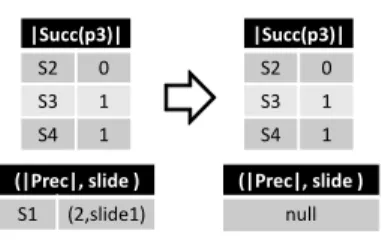
Before the window slides, the succeeding neighbor ofp3in three disparate ranges are
shown in Figure 4.1. After compared with all succeeding data points in the window of
Q1, there are no neighbors. Therefore it looks back to compare with data points in the
first slide. After found two neighbors which makep3 an unsafe inlier forQ1, forQ2 and
then Q3 it still has some succeeding data points not compared. So it keeps searching
in the non-overlapped slides contained by Q2 and thenQ3 in order until it hits the end
of the largest window. Meanwhile, for Q3 p3 becomes a safe inlier. All the succeeding
|Succ(p3)| S2 0 S3 1 S4 1 (|Prec|, slide ) S1 (2,slide1) |Succ(p3)| S2 0 S3 1 S4 1 (|Prec|, slide ) null
Figure 4.5: Arbitrary W: neighbor information
After the window slides,p13andp14arrive as new data points and p1 andp2 expire.
For Q1, we just need to add the neighbor numbers from slide 2 and 3 to see ifp3 is an
outlier. The same rule is applied toQ2. As for Q3 with the largest number,p3 is already
a safe inlier, therefore no need to do the search again. Accordingly, the safe indicator is
updated to 2 and unsafe is updated 2 indicating forQ1p3 is an outlier.
4.5
Varying Parameter - S
Assume all queries start simultaneously, consider the pattern-specific parameters and one of the window-specific parameters W are the same for the workload of a bunch of queries with different S values. This implies that all queries share the count, range, window size and require output at the same time, while outlier data points that need to be reported for each query differ.
Not like the previous cases where neighbors can be shared among all the queries in the workload, in this case, different slide sizes only influence the moving unit of each window sliding and the output timing of the outlier results. According to the characteristics of window mechanism, a window is triggered by certain time duration or certain number of arriving data points, then slides forward. Hence, each time how much a window slides depends on the slide size of the query specified by different users. Therefore in order to evaluate an appropriate value to enable the sharing among a workload with queries of arbitrary slide size, a greatest common divisor is calculated based on these different S
values. This greatest common divisor is then used as the smallest unit which we call slice for a window to move forward.
In terms of the features of greatest common divisor, each distinct slide size is divis-ible by the slice size. This important characteristic allows us to simply use a counter to measure number of times the slice size a window has slided and then to evaluate if the corresponding slide size has been hit. Once it comes up to the time that one specific slide size has been slided over, then outliers are outputted for queries with that slide size. All corresponding maintenances also update at this time. Each time window slides, counter increases its value up one and to see if there is any need to output. Also, if the counter is accumulated to the greatest slide size in the whole workload, reset is triggered and counting starts from the scratch.
4.6
Varying Parameter - W and S
Now we consider when both window-specific parameters change yet the pattern-specific parameters remain the same for all queries in the workload. This means that the count, range and require output at the same time are shared by all queries, while outlier data points that need to be reported for each query differ.
Case of multiple slide sizes and case of multiple window sizes are orthogonal struc-tures, so naturally combining those two strategies and data structures together does not cause heavy workload. This is because, for case of multiple window sizes, we can simpli-fy all the maintenance down to the progressive patterns in each slide, status indicator for the whole workload and the update trigger overheads. For case of multiple slide sizes, we only need to decide the timing we are required to output outliers and when to update cor-responding intermediate results. Consequently, as to each different slide size, we exploit their greatest common divisor as slice size, making slice the smallest unit we use to store
neighbor information. Therefore, case of arbitrary W and S can be regarded as arbitrary W case with fixed slide size whose value is slice size.
The pseudocode for the core routines is shown in Algorithm 3 and 4.
Algorithm 3SOP(pi,D) Arrival
Require: Data pointpi, DatasetD,W, slice //Dis Data points in the current window,Wis a set of different value of W
1: foreach q∈pi.succPoint(slice)do
2: if(true ==pi.isNeighbor(q)then
3: pi.—Succ(pi, slice)— ++; 4: pi.updateStatusIndicator; 5: if(pi.—Succ(pi,wmin)— ¿= k)then 6: break; 7: end if 8: end if 9: end for
10: whilepi.precSlides! =NULL and !pi.isSafedo
11: slide = getSlideWithLargestLifespan(pi.precSlides(slice));
12: foreach q∈slidedo
13: if(true ==pi.isNeighbor(q)then
14: pi.—Prec(pi,wmin)— ++;
15: slide.updateTriggeredList(pi);
16: if( (pi.—Prec(pi,wmin)— +pi.—Succ(pi,wmin)— ¿= k)then
17: break; 18: end if 19: pi.updateTriggeredSlide(slide); 20: pi.updateStatusIndicator; 21: end if 22: end for 23: end while
Algorithm 4SOP(pi,D) Departure
Require: Data pointpi, DatasetD,W, slice //Dis Data points in the current window,Wis a set of different value of W
1: foreachpi∈expSlide.triggereListdo
2: slide =pi.getUncomparedSlide(slice);
3: foreach q∈pi.succPoint(slide)do
4: if(true ==pi.isNeighbor(q)then
5: pi.—Succ(pi, slice)— ++; 6: pi.updateStatusIndicator; 7: if(pi.—Succ(pi,wmin)— ¿= k)then 8: break; 9: end if 10: end if 11: end for 12: pi.updateTriggeredSlide(slide); 13: pi.updateStatusIndicator; 14: end for
The first loop in the Algorithm 4 shows that we use slice as the smallest unit to slide the window. And every time we update the number of neighbors, the timing is based on size of slice. The body of the first loop in Algorithm 5 is for triggered potential outliers to find new neighbors. During the process, slice is the smallest unit all the time and be used
as a basic slide size.
4.7
Varying Parameter - K, R, W and S
Now we consider when both window-specific parameters and pattern-specific parameters change for all queries in the workload. This means that the count, range, required output at the same time and outlier data points that need to be reported for each query all differ. This is the general case that frequently happens in the real application.
We actually can utilize a combination of previously introduced techniques to achieve the maximum sharing. This is so because for the case of arbitrary pattern-specific parame-ters only, the maintenance and data structure it involves in mainly is related to the number of neighbors and corresponding update triggers. This means holding all the patterns iden-tified by them in a containment relationship. Yet for the case of arbitrary window-specific parameters only, all it refers to mainly is the size of the snapshot of the data streaming we are analyzing and the sliding frequency. Therefore, they are orthogonal from each other and can be integrated together without modification of sharing strategies and data structure.
4.8
Complexity Analysis
Computational Costs Computationally, there are two major actions that contribute to
the cost of neighbor searching. We recall that, first range query compares all the data points in the window no matter if these comparisons are necessary or not for each data point. Instead of expensive cost of range query, neighbor search of SOP stops once the query with the most restricted parameter specification is satisfied. Moreover, when one data point is searching neighbors in the window, all the other data points being compared
with also maintain the neighbor information, which reduces more CPU computation costs. From this perspective, neighbor search for each data point is a constant operation. Second the cost of sharing for each data point only requires on neighbor search. For each data point, status indicators are set to indicate which queries will output the data point as an outlier or not. Thus the cost of multiple queries in the workload can be reduced from O(nk) (k is the number of queries, and n is the number of data points in the window) to O(n). Third, as for the general case, we maintain a minimum set, an organized table, to figure out the minimum k for each different r so no extra computation would be occupied.
Memory Costs The memory costs of SOP depends mainly on two factors, the
re-lation we maintain for different range which depends on the number of queries and the intermediate computation results from the comparison of two different data points. Com-plexity wise, compared to non-sharing method, memory requirements are multiplied by the number of queries. SOP significantly decreases it via status sharing lemma to just one neighbor search. As for the sharing method in [2], most of the intermediate computation and event-based trigger update and maintenance are obviously reduced via least searching lemma.
ConclusionAs discussed above, SOP structure maintains a minimum object set and
also achieves least computation. Evidently, we do not need to hold the number of com-parisons of data points equivalent to the complete window size at any stage for computing if two data points are neighbors or not, rather once the data point is a safe inlier for al-l, comparison stops. This is a clear win over the exiting methods for multiple queries computations that need to utilize range query from scratch.
However, we observe that the resource requirements of SOP grow withNvalues, the
number of different parameter specifications. More specifically, since SOP always search-es to meet the most rsearch-estricted parameters specification and maintains a relation of different R value to keep number of neighbors in different ranges, its memory and CPU
Chapter 5
Sharing Among Queries with Predicate
Parameters
In the preliminary section, a complete query template with outlier parameters and predi-cate parameters is fully demonstrated. Sharing approach on pattern and window specific parameters have been deliberated in the last section already. Integration of capability of handling predicate parameters into SOP becomes the next problem so that SOP can be-come more robust and pragmatic in the real application. Therefore, in this section, we shift our focus to another half of our problem, i.e. the design of processing and opti-mization strategies for the shared predicates in a workload of outliers detection queries. We begin with the concept of two different sets. Next, we present the intuition and the methodology of the sharing strategies for each case.
Assume that we have a workload WL consisting of a set of outlier detection queries. Each outlier query have arbitrary selection predicates on both target and scope. According to the particular role of each of these two screened sets via application of two predicate parameters, as described in previously section, we classify these two sets into two cate-gories. For the one to see if these data points in it are outliers or not, we call the set of
these data points Target Set. For the one that data points are selected separately against
which to be compared with data points in Target Setto evaluate whether they are
neigh-bors of data points in Target Set or not, we call the set constituted by these data points
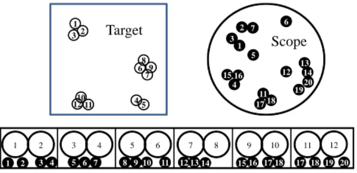
Scope Set. 3 4 2 1 5 6 7 8 910 11 121314 1516 1718 19 20 1 2 3 4 5 6 7 8 9 10 11 12 3 4 2 1 17 16 18 19 15 20 14 13 12 11 7 6 5 Scope 17 18 1 Target 2 3 45 689 7 10 11 12
Figure 5.1: Geographic Distribution and Window View
Figure 5.1 shows geography distribution and window view of both Target Set and
Scope Set. These two sets are composed of all data points specified by the corresponding
predicates given by the users. Target Set and Scope Set do not have to be pertaining to
each other. Nevertheless, from the perspective of the distance function, Target Set and
Scope Set should be related in some ways where connections are built on their meaning in the real world determined by the analysts. This can be perceived from the running example in problem formalization section. On the other hand, they can be the same data stream. D . . . Pn(D) P1(D) Multiple Predicates
Assume no sharing strategy is applied, then Figure 5.2 shows how method introduced earlier would process these requests. This helps to demonstrate conceptually that brute-force method causes huge inefficiency. In the first place each data point is sequenced by its time stamp when arriving system. Then based on different predicate, the input data stream D are divided into n subsets. All data points in one subset satisfies one particular predicate of one query. Thereafter, the outlier detection algorithm SOP is applied to each set of data points separately. Then for each query, the system outputs the corresponding correct result.
Simply applying SOP to each subset actually can meet the minimum demand that system can handle outlier detection queries with predicate parameters. However, usually most of predicate specifications have certain percentage of overlaps. If the workload contains a huge number of queries whose selections on this data stream differ subtly, then same computation of many times definitely wastes huge amounts of resources. Therefore, our goal in this section is to introduce sharing strategies that reduce these unnecessary costs.
5.1
Intuitions and Approaches
Given a continuous input stream, different queries in the workload will select disparate data points in it based on their own predicates. Therefore within a fixed window size, each
query maintains two lists of indexes pointing to the data points in Target Setand Scope
Set. These two lists dynamically update data points in it according to the expiration and
arrival of data points each time window slides.
Arbitrary Target PredicateThe main intuition for how we tackle the sharing
prob-lem for varying Target predicate is the following. Namely, we utilize the predicates p1,
sub-sets, called fragments in [3]. For each data point in each fragment, neighbors searching would be applied. In other words, a set of data points in a window of the input stream,
is partitioned into F0, F1, ..., Fk, a set of k + 1 disjoint fragments: D=F0∪F1∪... ∪Fk.
Each fragment Fi is associated with a subset of the workload WL that denoted by WL
(Fi) ¡ 2|W L|where every data point in the fragmentFi satisfies the predicates of every
query in WL (Fi), and no other query. Among all these fragments, the workload WL (F0)
is an empty set. This means that all data points inF0satisfy none of the predicates. Thus
none of these data points should participate in any query and accordingly can safely be ignored.
Meanwhile, a signature that identifies the precise subset of queries is associated with each data point. In other word, this signature of a data point encodes the fragment that it falls in and accordingly the query. This can be realized by using the bitmap to contain one bit for each of the n queries in the workload. Accordingly, when it comes to outputting timing for each query, outliers in different fragments can be aggregated in terms of the bitmap for different queries.
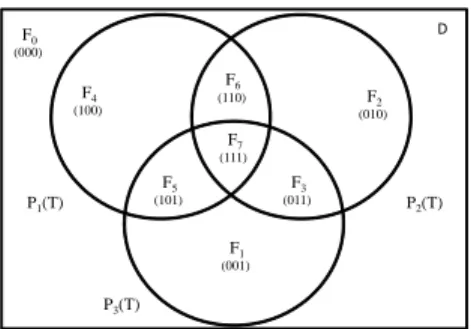
Example. Given a set of three queriesQ1,Q2 andQ3 with disparate Target predicate
predicatesp1,p2 andp3, how queries are related with each other by 8 fragments based on
these three predicates are shown in Figure 5.3. Also signatures for each fragment are also designated under the number of fragments.
F6 (110) F7 (111) D P1(T) F0 (000) F4 (100) (010)F2 F1 (001) F5 (101) F3 (011) P2(T) P3(T)
First we partition the Target Set into fragments. SOP can be applied in individual fragment to detect outliers. Then, we use an array to maintain this list of outliers in each fragment. Afterwards a simple add-up operation whose function is like an aggregation to accumulate all outliers in different fragments together for each query through looking up the signatures attached on those outliers. Therefore each data point just needs to apply
neighbor search once for queries with different Target Set but same Scope Set, which
significantly reduces the inefficiency aroused by repeated neighbor search. The basic idea of pipelining general outlier detection and aggregation is shown below.
D . . . Fk F1 O1(D) On(D) Fragment Filter Aggregation . . . . . . Fragments
Outlier Detection (SOP)
A
Figure 5.4: Conceptual View of Fragments Sharing
Arbitrary Scope Predicate In arbitrary Scope predicate case, we basically have a
similar intuition as in arbitrary Target predicate case. Given predicates p1,p2, p3, ...,pn
indicating different Scope predicates of queries in the workload, we partition the Scope data points from the input stream into disjoint subsets, called blocks. Namely these sets of data points in a window of the input stream are partitioned into a set of k disjoint
blocks: D =B0∪B1∪... ∪Bk. Each block is associated with a subset of the workload WL
that is denoted by WL (Bi) ¡2|W L| where every data point in the blockBi satisfies the
predicates of each query in WL (Bi), and no other query.
Nevertheless, in arbitrary Target case, it does not matter which fragment should be looked at first and which later. This is because all data points in different fragments have to be examined once if they are outliers or not. In arbitrary Scope case, we should
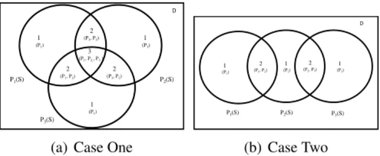
prior-2 (P1, P2) D P1(S) P2(S) P3(S) 1 (P1) 3 (P1, P2,, P3) 2 (P1, P2) 2 (P1, P2) 1 (P1) 1 (P1)
(a) Case One
D P1(S) P2(S) P3(S) 1 (P1) 2 (P1, P2) 2 (P2, P3) 1 (P3) 1 (P2) (b) Case Two
Figure 5.5: Possible Blocks in Two Different Case
itize the principle that once we find enough neighbors, then we stop searching neighbors to reduce the resources occupied by comparisons between two different data points to the minimum. If the bitmap signature used in arbitrary Target case is applied here, then like all data points in different fragments need to do neighbor search once, all data points in the blocks need to be probed against once. Therefore a different technique is utilized to distinguish different blocks.
In order to reduce the probing times by different queries over the same blocks, we tag each block a priority. This priority functions clarifying the overlap