Which Codes Have Cycle-Free Tanner Graphs? Tuvi Etzion, Senior Member, IEEE, Ari Trachtenberg, Student Member, IEEE, and Alexander Vardy,Fellow, IEEE
Abstract— If a linear block code of lengthn has a Tanner graph without cycles, then maximum-likelihood soft-decision decoding of can be achieved in timeO(n2). However, we show that cycle-free Tanner graphs cannot support good codes. Specifically, let be an(n; k; d) linear code of rateR = k=n that can be represented by a Tanner graph without cycles. We prove that ifR 0:5 then d 2, while if R < 0:5 then is obtained from a code of rate0:5 and distance 2 by simply repeating certain symbols. In the latter case, we prove that
d n k + 1 + n + 1 k + 1 < 2 R:
Furthermore, we show by means of an explicit construction that this bound is tight for all values ofn and k. We also prove that binary codes which have cycle-free Tanner graphs belong to the class of graph-theoretic codes, known as cut-set codes of a graph. Finally, we discuss the asymptotics for Tanner graphs with cycles, and present a number of open problems for future research.
Index Terms— Iterative decoding, linear codes, minimum distance, Tanner graphs.
I. INTRODUCTION
Iterative decoding algorithms on factor graphs [15] have become a subject of much active research in recent years [1], [2], [4], [5], [9], [15]–[18], [22], [29], and [30]. For example, the well-known turbo codes and turbo decoding methods [5], [4] constitute a special case of this general approach to the decoding problem. Factor-graph representations for turbo codes were introduced in [29] and [30], where it is also shown that turbo decoding is an instance of a general decoding procedure, known as the sum-product algorithm. Another extensively studied [8], [27] special case is trellis decoding of block and convolutional codes. It is shown in [9] and [30] that the Viterbi algorithm on a trellis is an instance of the min-sum iterative decoding procedure, when applied to a simple factor graph. The forward–backward algorithm on a trellis, due to Bahl, Cocke, Jelinek, and Raviv [3], is again a special case of the sum-product decoding algorithm. More general iterative algorithms on factor graphs, collectively termed the “generalized distributive law” or GDL, were studied by Aji and McEliece [1], [2]. These algorithms encompass maximum-likelihood decoding, belief propagation in Bayesian networks [10], [20], and fast Fourier trans-forms as special cases.
Manuscript received December 15, 1997; revised October 28, 1998. This work was supported by the David and Lucile Packard Foundation, the National Science Foundation, and the U.S.–Israel Binational Science Foundation under Grant 95-522. The work of A. Trachtenberg and A. Vardy was also supported by the Computational Science and Engineering Program at the University of Illinois. The material in this correspondence was presented in part at the IEEE International Symposium on Information Theory, MIT, Cambridge, MA, August 16–21, 1998.
T. Etzion is with the Department of Computer Science, Technion–Israel Institute of Technology, Haifa 32000, Israel.
A. Trachtenberg is with Digital Computer Laboratory, University of Illinois at Urbana-Champaign, Urbana, IL 61801 USA.
A. Vardy is with the University of California at San Diego, La Jolla, CA 92093-0428 USA.
Communicated by F. R. Kschischang, Associate Editor for Coding Theory. Publisher Item Identifier S 0018-9448(99)06101-5.
It is proved in [2], [15], [26], and [30] that the min-sum, the sum-product, the GDL, and other versions of iterative decoding on factor graphs all converge to the optimal solution if the underlying factor graph is cycle-free. If the underlying factor graph has cycles, very little is known regarding the convergence of iterative decoding methods.
This work is concerned with an important special type of factor graphs, known as Tanner1 graphs. The subject dates back to the work of Gallager [11] on low-density parity-check codes in 1962. Tanner [26] extended the approach of Gallager [11], [12] to codes defined by general bipartite graphs, with the two types of vertices representing code symbols and checks (or constraints), respectively. He also introduced the min-sum and the sum-product algorithms, and proved that they converge on cycle-free graphs. More recently, codes defined on sparse (regular) Tanner graphs were studied by Spielman [22], [25], who showed that such codes become asymptotically good if the underlying Tanner graph is a sufficiently strong expander. These codes were studied in a different context by MacKay and Neal [16], [18], who demonstrated by extensive experimentation that iterative decoding on Tanner graphs can approach channel capacity to within about 1 dB. Latest variants [17] of these codes come within about 0.3 dB from capacity, and outperform turbo codes.
In general, a Tanner graph for a code of length n over an alphabetA is a pair (G; L), where G = (V; E) is a bipartite graph andL = fC1; C2; 1 1 1 ; Crg is a set of codes over A, called behaviors
or constraints. We denote the two vertex classes ofG by X and Y, so thatV = X [ Y. The vertices of X are called symbol vertices and jX j = n, while the vertices of Y are called check vertices and jYj = r. There is a one-to-one correspondence between the constraintsC1; C2; 1 1 1 ; Cr inL and the check vertices y1; y2; 1 1 1 ; yr in Y; so that the length of the code Ci 2 L is equal to the degree
of the vertexyi2 Y, for all i = 1; 2; 1 1 1 ; r. A configuration is an assignment of a value fromA to each symbol vertex x1; x2; 1 1 1 ; xn
inX . Thus a configuration may be thought of as a vector of length n over A. Given a configuration = (1; 2; 1 1 1 ; n) and a vertex
y 2 Y of degree , we define the projection y of on y as a vector of length over A obtained from by retaining only those values that correspond to the symbol vertices adjacent to y. Specifically, iffxi ; xi ; 1 1 1 ; xi gX is the neighborhood of y in G; then y = (i ; i ; 1 1 1 ; i ). A configuration is said to be
valid if all the constraints are satisfied, namely, if y 2 Ci for all
i = 1; 2; 1 1 1 ; r. The code represented by the Tanner graph(G; L) is then the set of all valid configurations.
While the foregoing definition of Tanner graphs is quite general, the theory and practice of the subject [7], [16]–[18], [22], [26], is focused almost exclusively on the simple special case where all the constraints are single-parity-check codes over IF2. This work is no exception, although we will provide for the representation of linear codes over arbitrary fields by considering the zero-sum codes overIFq
rather than the binary single-parity-check codes. It seems appropriate
1Note on terminology. The term Tanner graph was first used by Wiberg, Loeliger, and K¨otter [30] to refer to the more general graphs introduced in [30]. These were later termed TWL graphs by Forney [9], although TWLK graphs would have been more appropriate. By now, the term factor graphs is almost universally used in this context, which leaves Tanner graphs available to refer to the kind of factor graphs actually studied by Tanner [26]. The emphasis in this paper (as in all of the literature [7], [16], [18], [22], and [26] on the subject) is on a special type of Tanner graphs that come with simple parity-check constraints. These Tanner graphs include the graphs underlying Gallager’s low-density parity-check codes [11], [12].
to call the corresponding Tanner graphs simple. Notice that in the case of simple Tanner graphs, the set of constraintsL is implied by definition, so that one can identify a simple Tanner graph with the underlying bipartite graphG. All of the Tanner graphs considered in this correspondence, except in Section V-C, are simple. Thus for the sake of brevity, we will henceforth omit the quantifier “simple.” Instead, when we consider the general case in Section V-C, we will use the term general Tanner graphs.
We can think of a (simple) Tanner graph for a binary linear code of length n as follows. Let H be an r 2 n parity-check matrix for . Then the corresponding Tanner graph for is simply the bipartite graph havingH as its X ; Y adjacency matrix. It follows that the number of edges in any Tanner graph for a linear code of lengthn is O(n2). Thus if we can represent by a Tanner graph without cycles, then maximum-likelihood decoding of can be achieved in timeO(n2), using the min-sum algorithm, for instance. However, both intuition and experimentation (cf. [16]) suggest that powerful codes cannot be represented by cycle-free Tanner graphs. The notion that cycle-free Tanner graphs can support only weak codes is, by now, widely accepted. Our goal in this correspondence is to make this “folk knowledge” precise. We provide rigorous answers to the question: Which codes can have cycle-free Tanner graphs?
Our results in this regard are two-fold: we derive a characterization of the structure of such codes and an upper bound on their minimum distance. The upper bound (Theorem 5) shows that codes with cycle-free Tanner graphs provide extremely poor tradeoff between rate and distance for each fixed length. This indicates that at very high signal-to-noise ratios these codes will perform badly. In general, however, the minimum distance of a code does not necessarily determine its performance at signal-to-noise ratios of practical interest. Indeed, there exist codes—for example, the turbo codes of [4] and [5]—that have low minimum distance, and yet perform very well at low signal-to-noise ratios. The development of analytic bounds on the performance of cycle-free Tanner graphs under iterative decoding is a challenging problem, which is beyond the scope of this work. Nevertheless, our results on the structure of the corresponding codes indicate that they are very likely to be weak: their parity-check matrix is much too sparse to allow for a reasonable performance even at low signal-to-noise ratios.
The rest of this correspondence is organized as follows. We start with some definitions and auxiliary observations in the next section. In Section III, we show that if an(n; k; d) linear code can be represented by a cycle-free Tanner graph and has rateR=k=n0:5; then d 2. We furthermore prove that if R < 0:5, then is necessarily obtained from a code of rate0:5 and minimum dis-tance2 by simply repeating certain symbols in each codeword. The-orem 5 of Section IV constitutes our main result: this theThe-orem gives an upper bound on the minimum distance of a general linear code that can be represented by a cycle-free Tanner graph. Furthermore, the bound of Theorem 5 is exact. This is also proved in Section IV by means of an explicit construction of a family of(n; k; d) linear codes that attain the bound of Theorem 5 for all values ofn and k. Asymptotically, forn ! 1, the upper bound takes the form
d 2b1=Rc (1)
and an immediate consequence of (1) is that asymptotically good codes with cycle-free Tanner graphs do not exist. We show in Section V that the same is true for Tanner graphs with cycles, unless the number of cycles increases exponentially with the length of the code. We also show in Section V that for every binary code that can be represented by a cycle-free Tanner graph, there exists a graph G such that is the dual of the cycle code of G. This establishes an interesting connection between codes with
cycle-(a) (b)
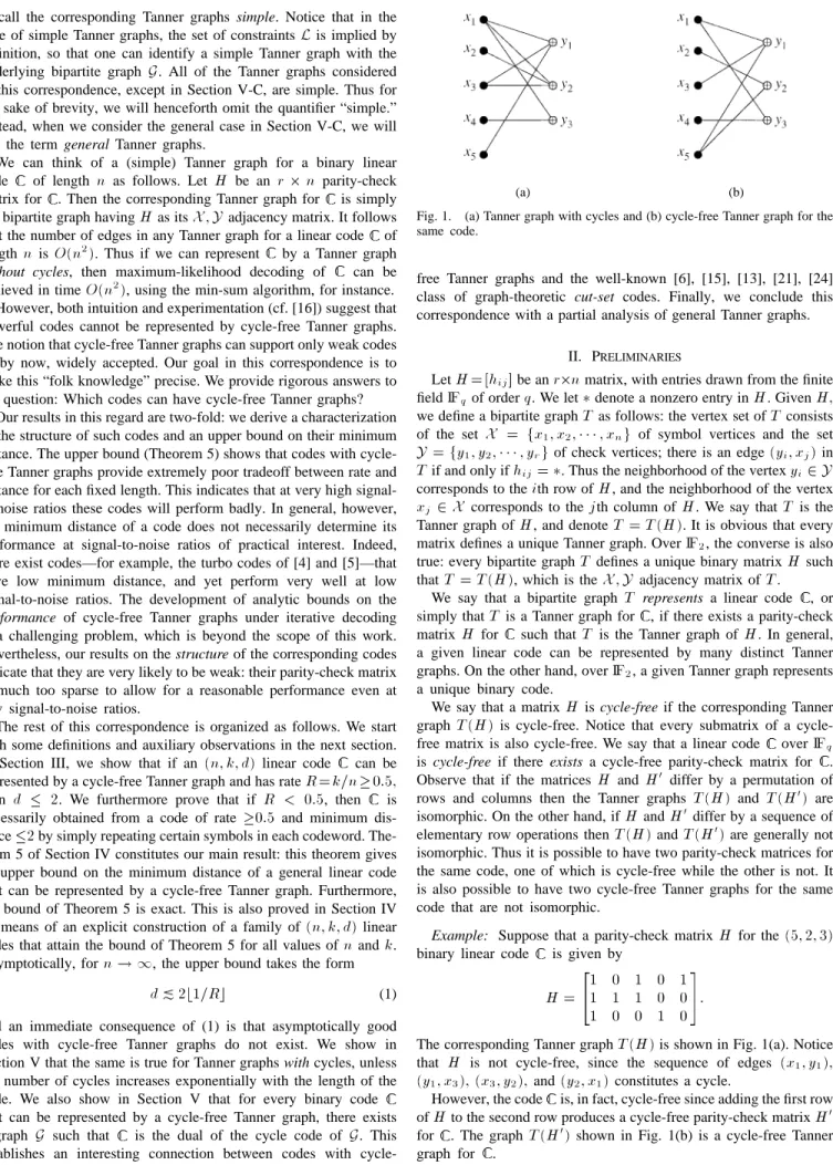
Fig. 1. (a) Tanner graph with cycles and (b) cycle-free Tanner graph for the same code.
free Tanner graphs and the well-known [6], [15], [13], [21], [24] class of graph-theoretic cut-set codes. Finally, we conclude this correspondence with a partial analysis of general Tanner graphs.
II. PRELIMINARIES
LetH =[hij] be an r2n matrix, with entries drawn from the finite
fieldIFqof orderq. We let 3 denote a nonzero entry in H. Given H; we define a bipartite graphT as follows: the vertex set of T consists of the set X = fx1; x2; 1 1 1 ; xng of symbol vertices and the set
Y = fy1; y2; 1 1 1 ; yrg of check vertices; there is an edge (yi; xj) in
T if and only if hij= 3. Thus the neighborhood of the vertex yi2 Y
corresponds to theith row of H, and the neighborhood of the vertex
xj 2 X corresponds to the jth column of H. We say that T is the
Tanner graph ofH, and denote T = T (H). It is obvious that every matrix defines a unique Tanner graph. OverIF2, the converse is also true: every bipartite graphT defines a unique binary matrix H such thatT = T (H), which is the X ; Y adjacency matrix of T .
We say that a bipartite graph T represents a linear code , or simply thatT is a Tanner graph for , if there exists a parity-check matrix H for such that T is the Tanner graph of H. In general, a given linear code can be represented by many distinct Tanner graphs. On the other hand, overIF2, a given Tanner graph represents a unique binary code.
We say that a matrixH is cycle-free if the corresponding Tanner graphT (H) is free. Notice that every submatrix of a cycle-free matrix is also cycle-cycle-free. We say that a linear code overIFq
is cycle-free if there exists a cycle-free parity-check matrix for . Observe that if the matricesH and H0 differ by a permutation of rows and columns then the Tanner graphs T (H) and T (H0) are isomorphic. On the other hand, ifH and H0 differ by a sequence of elementary row operations thenT (H) and T (H0) are generally not isomorphic. Thus it is possible to have two parity-check matrices for the same code, one of which is cycle-free while the other is not. It is also possible to have two cycle-free Tanner graphs for the same code that are not isomorphic.
Example: Suppose that a parity-check matrixH for the (5; 2; 3) binary linear code is given by
H = 1 0 1 0 11 1 1 0 0 1 0 0 1 0 :
The corresponding Tanner graphT (H) is shown in Fig. 1(a). Notice that H is not cycle-free, since the sequence of edges (x1; y1);
(y1; x3); (x3; y2); and (y2; x1) constitutes a cycle.
However, the code is, in fact, cycle-free since adding the first row ofH to the second row produces a cycle-free parity-check matrix H0 for . The graphT (H0) shown in Fig. 1(b) is a cycle-free Tanner graph for .
(a) (b)
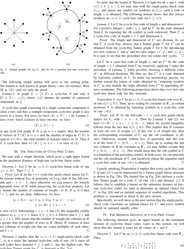
Fig. 2. Tanner graphs for (a)Enand (b) for a general low-rate cycle-free code.
The following simple lemma will serve as our starting point. This lemma is well known in graph theory—see, for instance, West [28, p. 52]—and we omit the proof.
Lemma 1: A graph G = (V; E) is cycle-free if and only if jEj = jV j 0 !(G), where !(G) denotes the number of connected
components inG.
A cycle-free graph consisting of a single connected component is called a tree, and thus a multiple-component cycle-free graph is also known as a forest. For trees, we havejEj = jV j 0 1 by Lemma 1. Since every forest contains at least one tree, we have
jEj jV j 0 1 (2)
for any cycle-free graph. IfM is an m 2 n matrix, then the number of vertices inT (M) is m + n and the number of edges in T (M) is equal towt (M)—the total number of nonzero entries in M. Thus if
M is cycle-free, then wt (M) m + n 0 1 in view of (2).
III. THESTRUCTURE OFCYCLE-FREECODES
We start with a simple theorem, which gives a tight upper bound on the minimum distance of high-rate cycle-free linear codes.
Theorem 2: Let be an(n; k; d) cycle-free linear code of rate
k=n 0:5. Then d 2.
Proof: LetH be the r2n cycle-free parity-check matrix for : We assume without loss of generality (w.l.o.g.) thatH has full row-rank and r = n 0 k, since otherwise we can remove the linearly dependent rows ofH while preserving the cycle-free property. Let
i denote the number of columns of weighti in H. If 06= 0 then
d = 1, and we are done. Otherwise, we have
1+ 2(n 0 1) = 1+ 2(2+ 3+ 1 1 1 + r)
wt (H) n + r 0 1 (3) in view of (2). Substitutingr = n 0 k into (3), this inequality readily reduces to1 k + 1. Since k=n 0:5, it follows that k r and
1 r +1. This means that the number of weight-one columns in H
is greater than the number of rows inH. Hence H contains at least two columns of weight one that are scalar multiples of each other, andd = 2.
Theorem 2 implies that the (n; n01; 2) single-parity-check code
Enis, in a sense, the optimal cycle-free code of rate0:5, since all such codes have distanced 2 and En has the highest rate. The cycle-free Tanner graph forEnis depicted in Fig. 2(a).
To show that the bound of Theorem 2 is tight for alln and k, with
n=2 k n 0 1, we may start with the single-parity-check code Ek+1 and repeat any symbol (or symbols) inEk+1 until a code of lengthn is obtained. The following lemma shows that this always produces an(n; k; 2) cycle-free code for k n=2.
Lemma 3: Let be a cycle-free code of lengthn and dimension k: Fix a positive integeri, with i n, and let 0be the code obtained from by repeating theith symbol in each codeword. Then 0 is a cycle-free code of lengthn + 1 and dimension k.
Proof: The length and dimension of 0 are obvious. To see that 0 is cycle-free, observe that a Tanner graph T0 for 0 can be obtained from the cycle-free Tanner graph T for by introducing two new verticesx0andy0and two new edges:(x0; y0) and (xi; y0).
It is easy to see that this procedure does not create new cycles. Let be a cycle-free code of length n, and let 3 be the code of lengthn + obtained from by iteratively applying times the procedure of Lemma 3, while possibly choosing a different value of i at different iterations. We then say that 3 is a code obtained by repeating symbols in . To make our terminology precise, we further extend the notion of codes obtained by “repeating symbols in ” to also include the codes obtained from 3by appending all-zero coordinates. The following proposition shows that every low-rate cycle-free linear code has this structure.
Proposition 4: Let be an(n; k; d) cycle-free linear code over IFq
of ratek=n 0:5. Then, up to scaling by constants in IFq at certain positions, is obtained by repeating symbols in a cycle-free code of rate >0:5.
Proof: Let H be the full-rank r 2 n cycle-free parity-check matrix for , with r = n 0 k. Then by Lemma 1 and (2), we have wt (H) n + r 0 1 3r 0 1, where the second inequality follows from the fact thatk=n 0:5. This implies that H contains at least one row of weight 2. If this row is of weight one, then the corresponding coordinate of , say the nth coordinate, is all-zero. Otherwise, assume without loss of generality that this row is of the form h = (0; 0; 1 1 1 ; 0; 3; 3). Then, up to scaling the last two columns ofH by constants in IFq, we may further assume that
h = (0; 0; 1 1 1 ; 0; 1; 01). This would mean that the nth symbol in
is a repetition of the preceding symbol. In both cases, we can puncture out thenth coordinate of , and iteratively repeat the argument until a cycle-free code of rate>0:5 is obtained.
Loosely speaking, Proposition 4 implies that every cycle-free code of rate0:5 can be represented by a Tanner graph whose structure is shown in Fig. 2(b). The dashed line in Fig. 2(b) encloses a cycle-free Tanner graph for a code 0 of rate >0:5 and distance 2. It follows that to establish a bound on the minimum distance of low-rate cycle-free codes, we need to determine an optimal choice for
0in Fig. 2(b) and an optimal sequence of symbol repetitions. This
problem is considered in detail in the next section.
Specifically, we will show in the next section that the single-parity-check code constitutes an optimal choice for 0, and every symbol should be repeated equally often.
IV. THEMINIMUMDISTANCE OFCYCLE-FREECODES The following theorem gives an upper bound on the minimum distance of cycle-free linear codes. Later in this section, we will show that this bound is exact for all values ofn and k.
Theorem 5: Let be an(n; k; d) cycle-free linear code over IFq. Then
(a) (b) (c) Fig. 3. (a) A cycle-free matrix, (b) its Tanner graph, and (c) its row-graph G.
Observe that fork=n 0:5, the bound in (4) reduces to d 2. This simple special case was dealt with in Theorem 2. The proof of Theorem 5 for generaln and k is considerably more involved. This proof will be presented in Section IV-B, after we establish a series of auxiliary lemmas in the next subsection.
A. Groundwork: Auxiliary Lemmas
For the sake of brevity, we will consider only binary codes, although our proof readily extends to codes over an arbitrary finite field. Furthermore, with a slight abuse of notation, we will not distinguish between equivalent codes: namely, given a parity-check matrixH for a code , we will often freely permute the columns ofH while still referring to the resulting matrix as a parity-check matrix for .
Let be an(n; k; d) cycle-free binary linear code, and let H be anr 2 n cycle-free parity-check matrix for , where r = n 0 k. We say thatH is in s-canonical form, if this matrix has the following structure:
H = A 0B I
s (5)
where all the rows ofB have weight 1, and Isis thes 2 s identity matrix, for somes in the range 0 s r. Notice that if s = 0 then (5) reduces toH = A (which means that every matrix is in
0-canonical form), while if s = r then the corresponding canonical
form isH = [B j Ir]. We will use the shorthand H = AksB to
denote thes-canonical form in (5).
Lemma 6: LetH =AksB be a cycle-free binary matrix in
s-canon-ical form, and suppose thats < r. Then at least one of the following statements is true.
The matrix A contains a row of weight two or less;
5 The matrix A contains three identical columns of weight one; ? The matrix A contains two identical columns of weight one, and
furthermore the row ofA which contains the nonzero entries of these two columns has weight three.
Proof: Let T (A) be the Tanner graph of A. Evidently T (A) is a subgraph of T (H), obtained by retaining only the first n 0 s symbol vertices x1; x2; 1 1 1 ; xn0s, the first r 0 s check vertices
y1; y2; 1 1 1 ; yr0s, and all the edges between these vertices. Since
T (H) is cycle-free by assumption, so is T (A). We now construct
another graph G, called the row-graph of A, whose vertex set
y1; y2; 1 1 1 ; yr0s corresponds to the rows ofA. The edge set of G is derived from the columns ofA of weight 2, so that a column of weightw in A contributes w 0 1 edges to G. An example illustrating the construction of the row-graphG for a 6 2 8 cycle-free matrix is depicted in Fig. 3.
Specifically, there is an edge betweenyiandyjinG iff i < j and there exists a column(a1; a2; 1 1 1 ; ar0s)tinA, such that ai= aj= 1
while ai+1 = ai+2 = 1 1 1 = aj01 = 0. Notice that each such
edge (yi; yj) in G corresponds to a path of length two in T (A):
namely(yi; xp); (xp; yj), where p denotes the position at which the column (a1; a2; 1 1 1 ; ar0s)t is to be found in A. It follows that if there is a cycle in G, then there is a cycle in T (A). Since T (A) is cycle-free, then so is G. As such, G necessarily contains at least two vertices of degree1, in view of (2). Let y3be one such vertex inG, and let a3= (a1; a2; 1 1 1 ; an0s) be the corresponding row of A.
Ifwt (a3) 2, then () is true. If wt (a3) = 3 and deg y3= 0, then
(5) is true. If wt (a3) = 3 and deg y3= 1, then (?) is true. Finally,
ifwt (a3) 4, then (5) is true, regardless of whether deg y3= 0 or
deg y3= 1.
We will say that anr 2 n matrix H is in reduced canonical form, ifH = AksB and either s = r or all the rows of A have weight 3.
Lemma 7: Let be an (n; k; d) cycle-free binary linear code. Then there exists a cycle-free parity-check matrix for , which is in reduced canonical form.
Proof: Let H be an arbitrary cycle-free parity-check matrix for . We first put H in s-canonical form, for the highest pos-sibles, by means of row and column permutations. This is achieved by considering all the rows ofH of weight one, for which the nonzero entry3 is contained in a column of weight one, and all the rows of
H of weight two such that at least one of the two 3 is contained in
a column of weight one. Under an appropriate column permutation, these rows ofH will form the submatrix [B j Is] in (5). If there
are no such rows, thens = 0 and H = A. Since row and column permutations preserve the cycle-free property ofH, this procedure produces a cycle-free parity-check matrixH0= AksB for , which
is in canonical form, although not necessarily reduced.
SinceH0= AksB is full-rank by assumption, all the rows of A
have weight 1. The key observation is that certain elementary operations on the rows of H0 allow us to eliminate rows of weight one and two inA, while still preserving the cycle-free property.
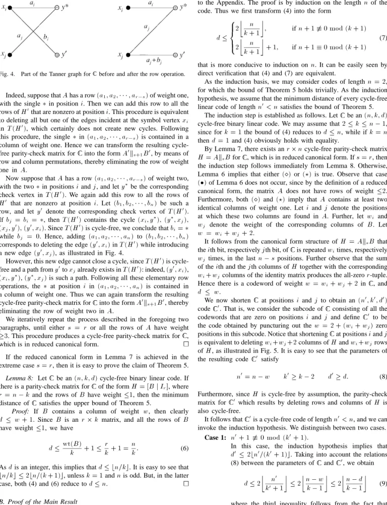
Fig. 4. Part of the Tanner graph for before and after the row operation.
Indeed, suppose thatA has a row (a1; a2; 1 1 1 ; ar0s) of weight one,
with the single3 in position i. Then we can add this row to all the rows ofH0that are nonzero at positioni. This procedure is equivalent to deleting all but one of the edges incident at the symbol vertexxi
in T (H0), which certainly does not create new cycles. Following this procedure, the single3 in (a1; a2; 1 1 1 ; ar0s) is contained in a
column of weight one. Hence we can transform the resulting cycle-free parity-check matrix for into the formA0ks+1B0, by means of row and column permutations, thereby eliminating the row of weight one in A.
Now suppose thatA has a row (a1; a2; 1 1 1 ; ar0s) of weight two,
with the two3 in positions i and j, and let y3be the corresponding check vertex in T (H0). We again add this row to all the rows of
H0 that are nonzero at position i. Let (b
1; b2; 1 1 1 ; bn) be such a
row, and lety0 denote the corresponding check vertex of T (H0). Ifbj = bi = 3, then T (H0) contains the cycle (xi; y3); (y3; xj);
(xj; y0); (y0; xi). Since T (H0) is cycle-free, we conclude that bi= 3
while bj = 0. Hence, adding (a1; a2; 1 1 1 ; an) to (b1; b2; 1 1 1 ; bn)
corresponds to deleting the edge(y0; xi) in T (H0) while introducing
a new edge(y0; xj), as illustrated in Fig. 4.
However, this new edge cannot close a cycle, sinceT (H0) is cycle-free and a path fromy0toxjalready exists inT (H0): indeed, (y0; xi),
(xi; y3), (y3; xj) is such a path. Following all these elementary row
operations, the 3 at position i in (a1; a2; 1 1 1 ; an) is contained in
a column of weight one. Thus we can again transform the resulting cycle-free parity-check matrix for into the formA0ks+1B0, thereby eliminating the row of weight two inA.
We iteratively repeat the process described in the foregoing two paragraphs, until either s = r or all the rows of A have weight
3. This procedure produces a cycle-free parity-check matrix for ,
which is in reduced canonical form.
If the reduced canonical form in Lemma 7 is achieved in the extreme cases = r, then it is easy to prove the claim of Theorem 5. Lemma 8: Let be an(n; k; d) cycle-free binary linear code. If there is a parity-check matrix for of the formH = [B j Ir], where
r = n 0 k and the rows of B have weight 1, then the minimum
distance of satisfies the upper bound of Theorem 5.
Proof: If B contains a column of weight w, then clearly d w + 1. Since B is an r 2 k matrix, and all the rows of B
have weight1, we have
d wt(B)k + 1 rk + 1 = nk: (6) Asd is an integer, this implies that d bn=kc. It is easy to see that
bn=kc 2bn=(k + 1)c, unless k = 1 and n is odd. But, in the latter
case, both (4) and (6) reduce tod n. B. Proof of the Main Result
We are now in a position to proceed with the proof of Theorem 5. Part of this proof involves tedious calculations, which will be deferred
to the Appendix. The proof is by induction on the length n of the code. Thus we first transform (4) into the form
d
2 k + 1n ; ifn + 1 6 0 mod (k + 1)
2 k + 1n + 1; ifn + 1 0 mod (k + 1) (7)
that is more conducive to induction onn. It can be easily seen by direct verification that (4) and (7) are equivalent.
As the induction basis, we may consider codes of lengthn = 2, for which the bound of Theorem 5 holds trivially. As the induction hypothesis, we assume that the minimum distance of every cycle-free linear code of lengthn0< n satisfies the bound of Theorem 5.
The induction step is established as follows. Let be an(n; k; d) cycle-free binary linear code. We may assume that2 k n 0 1, since fork = 1 the bound of (4) reduces to d n, while if k = n thend = 1 and (4) obviously holds with equality.
By Lemma 7, there exists anr 2 n cycle-free parity-check matrix
H = AksB for , which is in reduced canonical form. If s = r, then
the induction step follows immediately from Lemma 8. Otherwise, Lemma 6 implies that either (5) or (?) is true. Observe that case
() of Lemma 6 does not occur, since by the definition of a reduced
canonical form, the matrix A does not have rows of weight 2. Furthermore, both (5) and (?) imply that A contains at least two identical columns of weight one. Let i and j denote the positions at which these two columns are found in A. Further, let wi and
wj denote the weight of the corresponding columns of B. Let
w = wi+ wj+ 2.
It follows from the canonical form structure ofH = AksB that
theith bit, respectively jth bit, of is repeated witimes, respectively
wj times, in the lastn 0 s positions. Further observe that the sum of theith and the jth columns of H together with the corresponding
wi+ wjcolumns of the identity matrix produces the all-zeror-tuple. Hence there is a codeword of weight w = wi+ wj+ 2 in , and
d w.
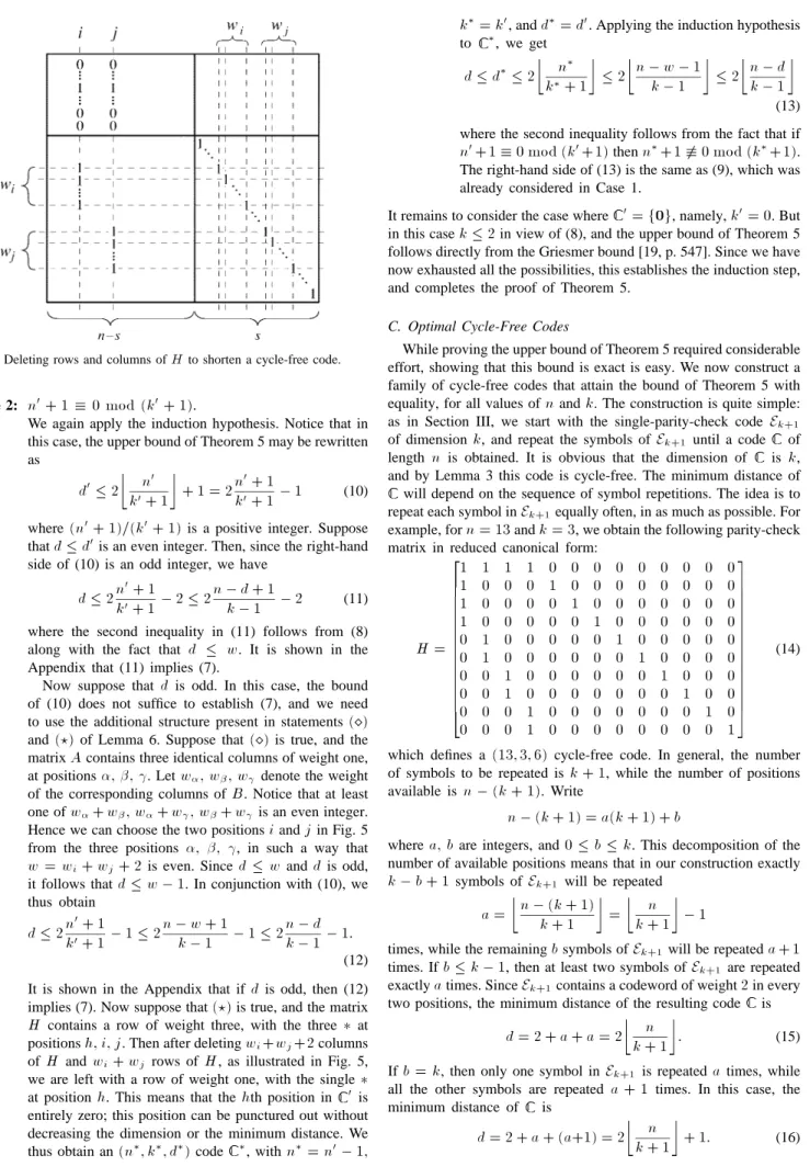
We now shorten at positionsi and j to obtain an (n0; k0; d0) code 0. That is, we consider the subcode of consisting of all the codewords that are zero on positions i and j and define 0 to be the code obtained by puncturing out the w = 2 + (wi+ wj) zero
positions in this subcode. Notice that shortening at positionsi and j is equivalent to deletingwi+wj+2 columns of H and wi+wjrows ofH, as illustrated in Fig. 5. It is easy to see that the parameters of the resulting code 0 satisfy
n0= n 0 w k0 k 0 2 d0 d: (8)
Furthermore, since H is cycle-free by assumption, the parity-check matrix for 0 which results by deleting rows and columns of H is also cycle-free.
It follows that 0is a cycle-free code of lengthn0< n, and we can invoke the induction hypothesis. We distinguish between two cases.
Case 1: n0+ 1 6 0 mod (k0+ 1):
In this case, the induction hypothesis implies that
d0 2bn0=(k0+ 1)c. Taking into account the relations
(8) between the parameters of and 0, we obtain
d 2 k0n+ 10 2 n 0 wk 0 1 2 n 0 dk 0 1 (9) where the third inequality follows from the fact that
d w. It is shown in the Appendix that the relation
Fig. 5. Deleting rows and columns ofH to shorten a cycle-free code.
Case 2: n0+ 1 0 mod (k0+ 1):
We again apply the induction hypothesis. Notice that in this case, the upper bound of Theorem 5 may be rewritten as
d0 2 n0
k0+ 1 + 1 = 2n 0+ 1
k0+ 10 1 (10)
where(n0+ 1)=(k0+ 1) is a positive integer. Suppose thatd d0is an even integer. Then, since the right-hand side of (10) is an odd integer, we have
d 2nk00+ 1+ 10 2 2n 0 d + 1k 0 1 0 2 (11) where the second inequality in (11) follows from (8) along with the fact that d w. It is shown in the Appendix that (11) implies (7).
Now suppose that d is odd. In this case, the bound of (10) does not suffice to establish (7), and we need to use the additional structure present in statements(5) and (?) of Lemma 6. Suppose that (5) is true, and the matrixA contains three identical columns of weight one, at positions; ; . Let w; w; wdenote the weight of the corresponding columns ofB. Notice that at least one ofw+ w; w+ w; w+ wis an even integer. Hence we can choose the two positionsi and j in Fig. 5 from the three positions ; ; , in such a way that
w = wi+ wj+ 2 is even. Since d w and d is odd,
it follows thatd w 0 1. In conjunction with (10), we thus obtain
d 2nk00+ 1+ 10 1 2n 0 w + 1k 0 1 0 1 2n 0 dk 0 1 0 1:
(12) It is shown in the Appendix that if d is odd, then (12) implies (7). Now suppose that(?) is true, and the matrix
H contains a row of weight three, with the three 3 at
positionsh; i; j. Then after deleting wi+wj+2 columns
of H and wi+ wj rows of H, as illustrated in Fig. 5, we are left with a row of weight one, with the single3 at position h. This means that the hth position in 0 is entirely zero; this position can be punctured out without decreasing the dimension or the minimum distance. We thus obtain an(n3; k3; d3) code 3, withn3= n00 1;
k3= k0, andd3= d0. Applying the induction hypothesis
to 3, we get
d d3 2 n3
k3+ 1 2 n 0 w 0 1k 0 1 2 n 0 dk 0 1
(13) where the second inequality follows from the fact that if
n0+1 0 mod (k0+1) then n3+1 6 0 mod (k3+1).
The right-hand side of (13) is the same as (9), which was already considered in Case 1.
It remains to consider the case where 0= f0g, namely, k0= 0. But in this casek 2 in view of (8), and the upper bound of Theorem 5 follows directly from the Griesmer bound [19, p. 547]. Since we have now exhausted all the possibilities, this establishes the induction step, and completes the proof of Theorem 5.
C. Optimal Cycle-Free Codes
While proving the upper bound of Theorem 5 required considerable effort, showing that this bound is exact is easy. We now construct a family of cycle-free codes that attain the bound of Theorem 5 with equality, for all values ofn and k. The construction is quite simple: as in Section III, we start with the single-parity-check code Ek+1
of dimensionk, and repeat the symbols of Ek+1 until a code of length n is obtained. It is obvious that the dimension of is k, and by Lemma 3 this code is cycle-free. The minimum distance of will depend on the sequence of symbol repetitions. The idea is to repeat each symbol inEk+1equally often, in as much as possible. For example, forn = 13 and k = 3, we obtain the following parity-check matrix in reduced canonical form:
H = 1 1 1 1 0 0 0 0 0 0 0 0 0 1 0 0 0 1 0 0 0 0 0 0 0 0 1 0 0 0 0 1 0 0 0 0 0 0 0 1 0 0 0 0 0 1 0 0 0 0 0 0 0 1 0 0 0 0 0 1 0 0 0 0 0 0 1 0 0 0 0 0 0 1 0 0 0 0 0 0 1 0 0 0 0 0 0 1 0 0 0 0 0 1 0 0 0 0 0 0 0 1 0 0 0 0 0 1 0 0 0 0 0 0 0 1 0 0 0 0 1 0 0 0 0 0 0 0 0 1 (14)
which defines a (13; 3; 6) cycle-free code. In general, the number of symbols to be repeated isk + 1, while the number of positions available is n 0 (k + 1). Write
n 0 (k + 1) = a(k + 1) + b
wherea; b are integers, and 0 b k. This decomposition of the number of available positions means that in our construction exactly
k 0 b + 1 symbols of Ek+1 will be repeated
a = n 0 (k + 1)k + 1 = k + 1n 0 1
times, while the remainingb symbols of Ek+1will be repeateda + 1 times. Ifb k 0 1, then at least two symbols of Ek+1are repeated exactlya times. Since Ek+1contains a codeword of weight2 in every two positions, the minimum distance of the resulting code is
d = 2 + a + a = 2 k + 1n : (15) Ifb = k, then only one symbol in Ek+1 is repeateda times, while all the other symbols are repeated a + 1 times. In this case, the minimum distance of is
(a) (b)
Fig. 6. Two alternative Tanner graphs for optimal cycle-free codes.
Notice thatb = k if and only if n + 1 0 mod (k + 1). Hence it follows from (15) and (16) that the code constructed in this manner attains the bound of Theorem 5 with equality.
Fig. 6 schematically shows two alternative cycle-free Tanner graphs for codes resulting from this construction (compare the Tanner graph in Fig. 6(a) with Fig. 2(b)).
We point out that although cycle-free codes obtained by repeating symbols inEk+1 have the highest possible minimum distance, they are not the only codes with this property. For example, consider the following parity-check matrix in reduced canonical form:
H = 1 1 1 0 0 0 0 0 0 0 0 0 0 1 0 0 1 1 0 0 0 0 0 0 0 0 0 1 0 0 0 1 0 0 0 0 0 0 0 0 1 0 0 0 0 1 0 0 0 0 0 0 0 0 1 0 0 0 0 1 0 0 0 0 0 0 0 1 0 0 0 0 0 1 0 0 0 0 0 0 0 1 0 0 0 0 0 1 0 0 0 0 0 0 1 0 0 0 0 0 0 1 0 0 0 0 0 0 1 0 0 0 0 0 0 1 0 0 0 0 0 1 0 0 0 0 0 0 0 1 : (17)
It is easy to see that this matrix defines a (13; 3; 6) cycle-free code 0, whose distance attains the bound of Theorem 5 with equality. This code was obtained by repeating symbols in a(5; 3; 2) code. It can be readily verified that 0 is not equivalent to the (13; 3; 6) cycle-free code , defined by the parity-check matrix in (14) and obtained by repeating symbols inE4. For instance, contains the all-one codeword, while 0 does not.
V. FURTHER RESULTS ANDOPENPROBLEMS
In this section, we discuss three different topics: a connection between binary cycle-free codes and cut-set codes of a graph, asymptotic behavior of Tanner graphs with cycles, and the extension of the results of the previous section to general Tanner graphs. In each case, we provide a number of open problems for future research.
A. Cycle-Free Codes and Graph-Theoretic Codes
There is an interesting connection between cycle-free codes and cut-set codes of a graph. LetG = (V; E) be a multigraph (a graph that may contain multiple edges with both endpoints the same) with
n = jEj edges and m = jV j vertices. A cut-set in G is a set of
edges which consists of all the edges having one endpoint in some setX V and the other endpoint in V n X. Under the operation of
(a) (b)
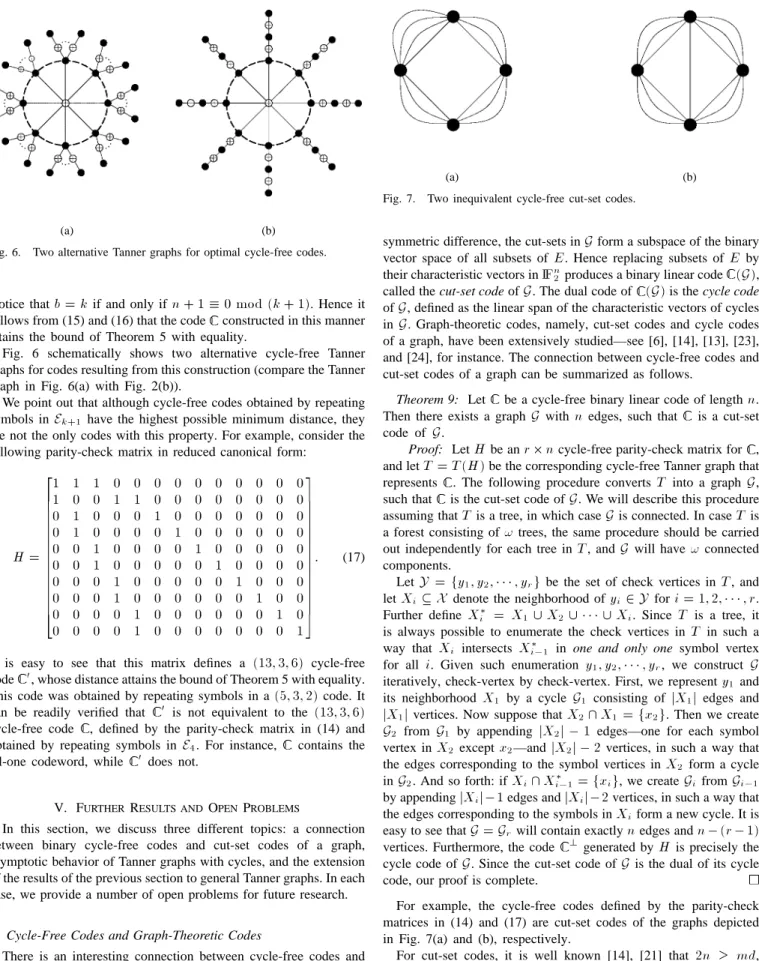
Fig. 7. Two inequivalent cycle-free cut-set codes.
symmetric difference, the cut-sets inG form a subspace of the binary vector space of all subsets of E. Hence replacing subsets of E by their characteristic vectors inIFn2produces a binary linear code (G), called the cut-set code ofG. The dual code of (G) is the cycle code ofG, defined as the linear span of the characteristic vectors of cycles in G. Graph-theoretic codes, namely, cut-set codes and cycle codes of a graph, have been extensively studied—see [6], [14], [13], [23], and [24], for instance. The connection between cycle-free codes and cut-set codes of a graph can be summarized as follows.
Theorem 9: Let be a cycle-free binary linear code of lengthn. Then there exists a graphG with n edges, such that is a cut-set code of G.
Proof: LetH be an r 2 n cycle-free parity-check matrix for , and letT = T (H) be the corresponding cycle-free Tanner graph that represents . The following procedure convertsT into a graph G, such that is the cut-set code ofG. We will describe this procedure assuming thatT is a tree, in which case G is connected. In case T is a forest consisting of! trees, the same procedure should be carried out independently for each tree inT , and G will have ! connected components.
LetY = fy1; y2; 1 1 1 ; yrg be the set of check vertices in T , and
letXi X denote the neighborhood of yi2 Y for i = 1; 2; 1 1 1 ; r.
Further define Xi3 = X1[ X2[ 1 1 1 [ Xi. Since T is a tree, it is always possible to enumerate the check vertices inT in such a way that Xi intersects Xi013 in one and only one symbol vertex for all i. Given such enumeration y1; y2; 1 1 1 ; yr, we construct G iteratively, check-vertex by check-vertex. First, we representy1and its neighborhood X1 by a cycle G1 consisting of jX1j edges and
jX1j vertices. Now suppose that X2\ X1= fx2g. Then we create
G2 from G1 by appending jX2j 0 1 edges—one for each symbol
vertex inX2 exceptx2—andjX2j 0 2 vertices, in such a way that
the edges corresponding to the symbol vertices inX2form a cycle inG2. And so forth: ifXi\ Xi013 = fxig, we create GifromGi01
by appendingjXij01 edges and jXij02 vertices, in such a way that
the edges corresponding to the symbols inXiform a new cycle. It is easy to see thatG = Grwill contain exactlyn edges and n 0 (r 0 1) vertices. Furthermore, the code ? generated byH is precisely the cycle code ofG. Since the cut-set code of G is the dual of its cycle code, our proof is complete.
For example, the cycle-free codes defined by the parity-check matrices in (14) and (17) are cut-set codes of the graphs depicted in Fig. 7(a) and (b), respectively.
For cut-set codes, it is well known [14], [21] that 2n md, wherem is the number of vertices in the underlying graph G. Indeed, this follows immediately from the fact that if the minimum distance of (G) is d, then every vertex of G must have degree at least d, otherwise, the cut-set that isolates this vertex will have less than
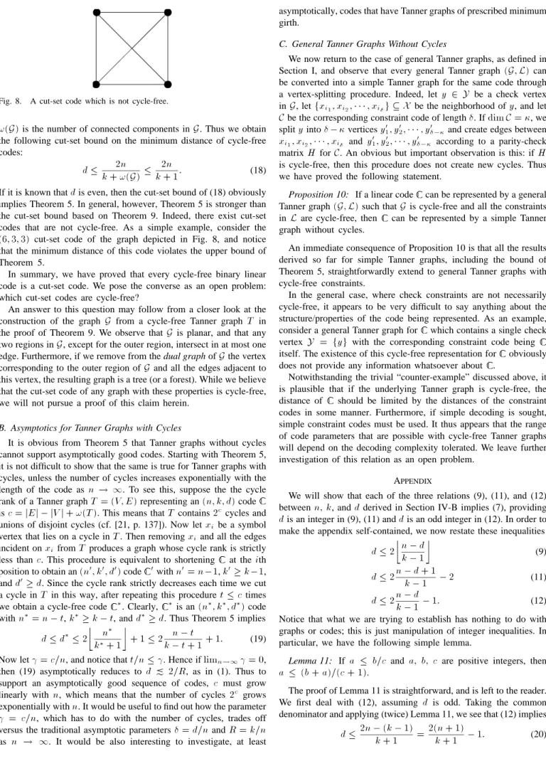
Fig. 8. A cut-set code which is not cycle-free.
!(G) is the number of connected components in G. Thus we obtain
the following cut-set bound on the minimum distance of cycle-free codes:
d k + !(G)2n 2nk + 1: (18) If it is known thatd is even, then the cut-set bound of (18) obviously implies Theorem 5. In general, however, Theorem 5 is stronger than the cut-set bound based on Theorem 9. Indeed, there exist cut-set codes that are not cycle-free. As a simple example, consider the
(6; 3; 3) cut-set code of the graph depicted in Fig. 8, and notice
that the minimum distance of this code violates the upper bound of Theorem 5.
In summary, we have proved that every cycle-free binary linear code is a cut-set code. We pose the converse as an open problem: which cut-set codes are cycle-free?
An answer to this question may follow from a closer look at the construction of the graphG from a cycle-free Tanner graph T in the proof of Theorem 9. We observe thatG is planar, and that any two regions inG, except for the outer region, intersect in at most one edge. Furthermore, if we remove from the dual graph ofG the vertex corresponding to the outer region ofG and all the edges adjacent to this vertex, the resulting graph is a tree (or a forest). While we believe that the cut-set code of any graph with these properties is cycle-free, we will not pursue a proof of this claim herein.
B. Asymptotics for Tanner Graphs with Cycles
It is obvious from Theorem 5 that Tanner graphs without cycles cannot support asymptotically good codes. Starting with Theorem 5, it is not difficult to show that the same is true for Tanner graphs with cycles, unless the number of cycles increases exponentially with the length of the code asn ! 1. To see this, suppose the the cycle rank of a Tanner graphT = (V; E) representing an (n; k; d) code isc = jEj 0 jV j + !(T ). This means that T contains 2c cycles and unions of disjoint cycles (cf. [21, p. 137]). Now letxibe a symbol vertex that lies on a cycle inT . Then removing xiand all the edges incident onxifromT produces a graph whose cycle rank is strictly less thanc. This procedure is equivalent to shortening at the ith position to obtain an(n0; k0; d0) code 0withn0= n01, k0 k01, andd0 d. Since the cycle rank strictly decreases each time we cut a cycle inT in this way, after repeating this procedure t c times we obtain a cycle-free code 3. Clearly, 3is an(n3; k3; d3) code withn3= n 0 t, k3 k 0 t, and d3 d. Thus Theorem 5 implies
d d3 2 n3
k3+ 1 + 1 2 n 0 tk 0 t + 1+ 1: (19)
Now let = c=n, and notice that t=n . Hence if limn!1 = 0,
then (19) asymptotically reduces tod 2=R, as in (1). Thus to support an asymptotically good sequence of codes, c must grow linearly withn, which means that the number of cycles 2c grows exponentially withn. It would be useful to find out how the parameter
= c=n, which has to do with the number of cycles, trades off
versus the traditional asymptotic parameters = d=n and R = k=n as n ! 1. It would be also interesting to investigate, at least
asymptotically, codes that have Tanner graphs of prescribed minimum girth.
C. General Tanner Graphs Without Cycles
We now return to the case of general Tanner graphs, as defined in Section I, and observe that every general Tanner graph (G; L) can be converted into a simple Tanner graph for the same code through a vertex-splitting procedure. Indeed, let y 2 Y be a check vertex inG, let fxi ; xi ; 1 1 1 ; xi g X be the neighborhood of y, and let
C be the corresponding constraint code of length . If dim C = , we
splity into 0 vertices y10; y02; 1 1 1 ; y00 and create edges between
xi ; xi ; 1 1 1 ; xi and y01; y02; 1 1 1 ; y00 according to a parity-check matrixH for C. An obvious but important observation is this: if H is cycle-free, then this procedure does not create new cycles. Thus we have proved the following statement.
Proposition 10: If a linear code can be represented by a general Tanner graph(G; L) such that G is cycle-free and all the constraints in L are cycle-free, then can be represented by a simple Tanner graph without cycles.
An immediate consequence of Proposition 10 is that all the results derived so far for simple Tanner graphs, including the bound of Theorem 5, straightforwardly extend to general Tanner graphs with cycle-free constraints.
In the general case, where check constraints are not necessarily cycle-free, it appears to be very difficult to say anything about the structure/properties of the code being represented. As an example, consider a general Tanner graph for which contains a single check vertex Y = fyg with the corresponding constraint code being itself. The existence of this cycle-free representation for obviously does not provide any information whatsoever about .
Notwithstanding the trivial “counter-example” discussed above, it is plausible that if the underlying Tanner graph is cycle-free, the distance of should be limited by the distances of the constraint codes in some manner. Furthermore, if simple decoding is sought, simple constraint codes must be used. It thus appears that the range of code parameters that are possible with cycle-free Tanner graphs will depend on the decoding complexity tolerated. We leave further investigation of this relation as an open problem.
APPENDIX
We will show that each of the three relations (9), (11), and (12) betweenn; k, and d derived in Section IV-B implies (7), providing
d is an integer in (9), (11) and d is an odd integer in (12). In order to
make the appendix self-contained, we now restate these inequalities
d 2 n 0 dk 0 1 (9)
d 2n 0 d + 1
k 0 1 0 2 (11)
d 2n 0 dk 0 1 0 1: (12) Notice that what we are trying to establish has nothing to do with graphs or codes; this is just manipulation of integer inequalities. In particular, we have the following simple lemma.
Lemma 11: If a b=c and a; b; c are positive integers, then a (b + a)=(c + 1).
The proof of Lemma 11 is straightforward, and is left to the reader. We first deal with (12), assuming d is odd. Taking the common denominator and applying (twice) Lemma 11, we see that (12) implies
d 2n 0 (k 0 1)
Since(d + 1)=2 is an integer for odd d, it follows from (20) that
(d + 1)=2 b(n+1)=(k+1)c. This may be rewritten as
d 2 n + 1k + 1 0 1: (21) Ifn + 1 6 0 mod (k + 1) then b(n + 1)=(k + 1)c = bn=(k + 1)c, and (21) clearly implies (7). If(n + 1)=(k + 1) is an integer, then (21) is precisely the equivalent form of (7) given in (10).
It is easy to see that ifd is an odd integer, then (9) implies (12). Since this case was already established above, it remains to prove (9) for evend. Using once again Lemma 11, we see that (9) implies
d 2n=(k + 1), or equivalently d=2 n=(k + 1). Since d=2 is an
integer for evend, we can take the integer part of n=(k + 1) in the above expression. It follows that for evend, we have
d 2 k + 1n
which clearly implies (7). Finally, it can be readily seen that ifd is an integer, then (11) implies (9). Hence, our proof of Theorem 5 is now complete.
ACKNOWLEDGMENT
The authors are grateful to Jeff Erickson, Amir Khandani, and Ralf K¨otter for stimulating discussions. The authors would also like to thank the anonymous referees for their valuable comments, which improved the presentation of this correspondence.
REFERENCES
[1] S. M. Aji and R. J. McEliece, “A general algorithm for distributing information in a graph,” in Proc. IEEE Int. Symp. Information Theory (Ulm, Germany, 1997), p. 6.
[2] S. M. Aji and R. J. McEliece, “The generalized distributive law,” IEEE Trans. Inform. Theory, submitted for publication, July 1998.
[3] L. R. Bahl, J. Cocke, F. Jelinek, and J. Raviv, “Optimal decoding of linear codes for minimizing symbol error rate,” IEEE Trans. Inform. Theory, vol. IT-20, pp. 284–287, 1974.
[4] C. Berrou and A. Glavieux, “Near optimum error correcting coding and decoding: Turbo-codes,” IEEE Trans. Commun., vol. 44, pp. 1261–1271, 1996.
[5] C. Berrou, A. Glavieux, and P. Thitimajshima, “Near Shannon limit error-correcting coding and decoding: Turbo codes,” in Proc. IEEE Int. Conf. Communications (Geneva, Switzerland, 1993), pp. 1064–1070. [6] J. Bruck and M. Blaum, “Neural networks, error-correcting codes, and
polynomials over the binaryn-cube,” IEEE Trans. Inform. Theory, vol. 35, pp. 976–987, 1989.
[7] M. Esmaeili and A. K. Khandani, “Acyclic Tanner graphs and maximum-likelihood decoding of linear block codes,” preprint, May 1998.
[8] J. Feigenbaum, G. D. Forney Jr., B. H. Marcus, R. J. McEliece, and A. Vardy, Eds., Special Issue on “Codes and Complexity,” IEEE Trans. Inform. Theory, vol. 42, pp. 1649–2064, Nov. 1996.
[9] G. D. Forney Jr., “The forward-backward algorithm,” in Proc. 34th Allerton Conf. Communication, Control, and Computing (Monticello, IL., Oct. 1996), pp. 432–446.
[10] B. J. Frey, “Bayesian networks for pattern classification, data compres-sion, and channel coding,” Ph.D. dissertation, Univ. Toronto, Toronto, Ont., Canada, July 1997.
[11] R. G. Gallager, “Low-density parity-check codes,” IRE Trans. Inform. Theory, vol. IT-8, pp. 21–28, 1962.
[12] R. G. Gallager, Low-Density Parity-Check Codes. Cambridge, MA: MIT Press, 1963.
[13] S. L. Hakimi and J. Bredeson, “Graph theoretic error-correcting codes,” IEEE Trans. Inform. Theory, vol. IT-14, pp. 584–591, 1968.
[14] S. L. Hakimi and H. Frank, “Cut-set matrices and linear codes,” IEEE Trans. Inform. Theory, vol. IT-11, pp. 457–458, 1965.
[15] F. R. Kschischang, B. J. Frey, and H.-A. Loeliger, “Factor graphs and the sum-product algorithm,” IEEE Trans. Inform. Theory, submitted for publication, July 1998.
[16] D. J. C. MacKay, “Good error-correcting codes based on very sparse matrices,” IEEE Trans. Inform. Theory, vol. 45, pp. 399–431, Mar. 1999. [17] , “Gallager codes that are better than turbo codes,” in Proc. 36th Allerton Conf. Communication, Control, and Computing (Monticello, IL., Sept. 1998).
[18] D. J. C. MacKay and R. M. Neal, “Near Shannon limit performance of low-density parity-check codes,” Electron. Lett., vol. 32, pp. 1645–1646, 1996.
[19] F. J. MacWilliams and N. J. A. Sloane, The Theory of Error-Correcting Codes. New York: North-Holland, 1977.
[20] J. Pearl, Probabilistic Reasoning in Intelligent Systems: Networks of Plausible Inference. San Mateo, CA: Kaufmann, 1988.
[21] W. W. Peterson and E. J. Weldon Jr., Error-Correcting Codes, 2nd ed. Cambridge, MA: MIT Press, 1961.
[22] M. Sipser and D. A. Spielman, “Expander codes,” IEEE Trans. Inform. Theory, vol. 42, pp. 1710–1722, 1996.
[23] P. Sol´e and T. Zaslavsky, “The covering radius of the cycle code of a graph,” Discr. Appl. Math., vol. 45, pp. 63–70, 1993.
[24] , “A coding approach to signed graphs,” SIAM J. Discr. Math., vol. 7, pp. 544–553, 1994.
[25] D. A. Spielman, “Linear-time encodable and decodable codes,” IEEE Trans. Inform. Theory, vol. 42, pp. 1723–1731, 1996.
[26] R. M. Tanner, “A recursive approach to low-complexity codes,” IEEE Trans. Inform. Theory, vol. IT-27, pp. 533–547, 1981.
[27] A. Vardy, “Trellis structure of codes,” in Handbook of Coding Theory, V. S. Pless and W. C. Huffman, Eds. Amsterdam, The Netherlands: Elsevier, 1998, pp. 1989–2118.
[28] D. B. West, Introduction to Graph Theory Englewood Cliffs, NJ: Prentice-Hall, 1996.
[29] N. Wiberg, “Codes and decoding on general graphs,” Ph.D. dissertation, Dep. Elec. Eng., Univ. Link¨oping, Link¨oping, Sweden, Apr. 1996. [30] N. Wiberg, H.-A. Loeliger, and R. K¨otter, “Codes and iterative decoding
on general graphs,” Euro. Trans. Telecommun., vol. 6, pp. 513–526, 1995.
Time-Varying Periodic Convolutional Codes With Low-Density Parity-Check Matrix
Alberto Jim´enez Felstr¨om,Member, IEEE, and Kamil Sh. Zigangirov,Senior Member, IEEE
Abstract—We present a class of convolutional codes defined by a low-density parity-check matrix and an iterative algorithm of the decoding of these codes. The performance of this decoding is close to the performance of turbo decoding. Our simulation shows that for the rate R = 1=2 binary codes, the performance is substantionally better than for ordinary convolutional codes with the same decoding complexity per information bit. As an example, we constructed convolutional codes with memory
M = 1025; 2049; and 4097 showing that we are about 1 dB from
the capacity limit at a bit-error rate (BER) of 1005 and a decoding complexity of the same magnitude as a Viterbi decoder for codes having memory M = 10.
Index Terms— Convolutional codes, iterative decoding, low-density parity-check codes.
Manuscript received June 19, 1997; revised March 20, 1999. The material in this correspondence was presented in part at the International Symposium on Information Theory, Cambridge, MA, August 16–21, 1998.
The authors are with the Telecommunication Theory Group, Department of Information Technology, Lund University, S-221 00, Lund, Sweden (e-mail: [email protected]).
Communicated by N. Seshadri, Associate Editor for Coding Techniques. Publisher Item Identifier S 0018-9448(99)05867-8.