A Neural Learning Algorithm of Blind Separation of Noisy Mixed Images Based on Independent Component Analysis

A Neural Learning Algorithm of Blind Separation

of Noisy Mixed Images Based on Independent

Component Analysis

Hongyan Li

College of Information Engineering of Taiyuan University of Technology, Taiyuan,China E-mail: [email protected]

Xueying Zhang

College of Information Engineering of Taiyuan University of Technology, Taiyuan,China E-mail: [email protected]

Abstract—Blind source separation problem has recently received a great deal of attention in signal processing and unsupervised neural learning. In the current approaches, the additive noise is negligible so that it can be omitted from the consideration. To be applicable in realistic scenarios, blind source separation approaches should deal evenly with the presence of noise. In this contribution, we proposed approaches to independent component analysis when the measured signals are contaminated by additive noise. A noisy multiple channels neural learning algorithm of blind separation is proposed based on independent component analysis. The data have no noise are used to whiten the noisy data, and the windage wipe off technique is used to correct the infection of noise, a neural network model having denoise capability is adopted to recover some original signals from their noisy mixtures observed by the same number of sensors. And a relaxation factor is introduced into the iteration algorithm, thus the new algorithm can implement convergence. Computer simulations and experiment results prove the feasibility and validity of the neural network modeling and control method based on independent component analysis, which can renew the original images effectively.

Index Terms—Independent component analysis; Neural network; Blind source separation; Noise cancellation; Relaxation factor

I. INTRODUCTION

Independent component analysis (ICA) is a statistical technique in signal processing and machine learning that aims at finding linear projections of the data that maximize their mutual independence. The process of ICA is extracting unknown independent source signals from sensor that are unknown combinations of the source signals. The work has been one of the most exciting topics in the fields of neural computation, advanced statistics, signal processing, and communication engineering which find independent components from observing multidimensional data based on higher order statistics[1~4].

Blind source separation is a technique that extracts the original signals from their mixtures observed by

sensors. In order to solve the problem of blind signal separation, many techniques have been proposed [5~9]. Among them, the ICA methods are based on the assumption of mutual independence of the sources. Traditional ICA has some assumption such as assuming that there is no noise or noise is minute that can be ignored, so it can not solve the problem of the noisy blind signal separation. Most of ICA methods are developed in the case of noiseless data. Some fast and efficient algorithms have been proposed such as FASTICA [10~14]. However, all these algorithms perform poorly when noise affects the data. To overcome the ICA limitation, some work has been done to partially overcome this limitation [15~19]. An earlier research of this paper has been done in [20], which combined ICA and neural network to separate the noisy mixed speech. Moreover, in this paper, considering that the negative gradient direction is the fastest decline of the function value, thus, we select the gradient value as the relaxation factor, and the relaxation factor is introduced into the iteration algorithm to improve the convergence, and a improved noisy multiple channels neural learning algorithm of blind separation combining with windage wipe off technique is proposed to solve the problem of noisy multiple blind signal separation. As well as the proposed algorithm is applied in the noisy multiple channels blind images sources separation. Finally, more conclusions and analysis are presented in the simulations. Separation results obtained from test demonstrate the feasibility of our approach.

blind separation algorithms. Finally, conclusions and analysis are presented in section 5.

II ICARECURRENT NEURAL NETWORK STRUCTURE

ICA is one method for performing blind signal separation that aims to recover unknown sources from a set of their observations, in which they are mixed in an unknown manner. Suppose that signals sj(t) (j=1,2,…,n) are generated by n statistically independent sources, and their linear mixtures xi(t) (i=1,2,…,n) are observed by n sensors:

( )

t a

( ) ( )

t s t

x n _j

j ij i

∑

= = 1 (1)

where aij are constants independent of time t.

The aim of ICA is to find the matrix W, The ICA recurrent neural network structure can be depicted by Fig.1 [21].

Improving this model with a whole connected recurrent neural network, each neuron is connected with the whole neurones, the model can be expressed as

( )

t x

( )

t w

( ) ( )

t y t

y j n j ij i i

∑

= − = 1 (2)

With the optimal weight wij,the output signals can be independent mutually. The independent vectors f(x) and g(x) have the formula

( ) ( )

[f x g x ] E[f( )x ]E[g( )x ]

E =

(3)

Fig.1 ICA recurrent neural network structure

Supposing that the independent signal yi and yj are zero mean, the generalized covariance matrix of the non-linear transform f (yi) and f (yj) are nonsingular diagonal matrix, that is

( ) ( )

[

]

[

( )

]

[

( )

]

( ) ( )

[

]

[

( )

]

[

( )

]

( ) ( )

[

]

[

( )

]

[

( )

]

⎥⎥ ⎥ ⎦ ⎤ − ⎢ ⎢ ⎢ ⎣ ⎡ − = − = n n n n fg y g E y f y g y f y g E y f E y g y f E g E f E g f E R E E 0 0 1 1 1 1 T T % % y y y y

(4) where the covariance E

[

f

( )

y_i g

( )

y_j

]

−E

[

f

( )

y_i

]

E

[ ]

g

( )

y_j

is zero when i is not equal to j, the variance

( ) ( )

[

f yi gyi

]

E

[

f

( )

yi

]

E

[ ]

g

( )

yi

E − is not zero, and f(y) and g(y) are different nonlinear activation function.

According to the statistic independence and the normalize condition E

[

f

( ) ( )

y_i g y_i

]

=_λi , the real-time learning algorithm can be deduced

( )

_{( )}

_[

_{[ ]}

_{( )}

_{[ ]}

_{( )}

_]

( )

_{( )}

_{[ ]}

_{( )}

_{[ ]}

_{( )}

⎪ ⎪ ⎩ ⎪⎪ ⎨ ⎧ ≠ = − = j i t y g t y f t dt t w t y g t y f t dt t w j i ij i i i ii μ λ μ d d (5)

It can be expressed as matrix form

( )

_{( )}

_t

_[

_f

_{[ ]}

_{( )}

_{t g}

_{[ ]}

_{( )}

_t

_]

t t y y Λ W T d d −

=μ (6)

where Λ=diag

{

_λ1,_λ2,",_λn

}

III A NOISY MULTIPLE CHANNELS BLIND SIGNAL

SEPARATION ALGORITHM BASED ON NEURAL NETWORK

For the noisy ICA model x=As+n, the hypothesis are showed as follows

1) The noise and the independent component are independent mutually

2) The covariance of noise is foregone 3) n is Gaussian noise

In the presence of noise, ICA becomes quite difficulty, the biggest difficult problem is how to estimate the independent component without noise. Estimating the noise component becomes more difficult because the noise model is not reversible. We reduce the effects of noise from three aspects, first of all, in pre-processing, noise effects are considered in the whitening of the data, the data having no noise are used to whiten the noisy data, in addition, the windage wipe off technique is used to correct the infection of noise, at last, a ICA model based on clustering algorithm of neural network having denoise capability as well as a relaxation factor is introduced into the iteration algorithm to improve the convergence and realize the noisy multiple channels blind source separation.

A The Whitening of Data

The ICA problem is greatly simplified if the observed mixture vectors are first whitened or sphered. A zero-mean random vector x=(x1,…,xn)T is said to be

#

training

#

#

∑ ∑ ∑ ∑

s1(t) x1(t)

sn(t) xn(t) _yn(t)

y1(t) a11

a1n

an1

ann

wn1 w1n

white if its elements xi are uncorrelated and have unit

variances. If the centralized signal is x, the whitened signal is

x

~

, in terms of the covariance matrix, that means

[ ]

x~x~T =I

E

(7)

where I is the unit matrix.

It is easy to see that the whitening signals have unit variance and uncorrelated, independently of the rotation angle. The whitening has a solution using eigenvalue decomposition for the covariance matrix of signals. Let V be the orthogonal matrix consisted of covariance matrix_E

[ ]

_xxT _{. Let diag( , , )}

1 dn d "

=

D be the diagonal

matrix of the eigenvalue of _E

[ ]

_xxT _{, the whitening}

process can be described as

( )

t VD V x

( )

t

x 1/2 T

~ ₌ − ₍₈₎

Making that _{U =VD}−1/2_VT_{, where U is the whitening}

matrix which is usually computed after singular or eigenvalue decomposition of the covariance matrix ofx(t),that is

( )

t Ux

( )

t x =

~ ₍₉₎

where

_x

~

( )

_t

is the whitened mixing signal.

If we replace x=As into Eq.(4) and make A~=UA, the formula becomes

( )

t UAs

( )

t As

( )

t

x ~

~ _{= = (10)}

where

A

~

is a global mixing matrix.

Supposing that the covariance matrix of noise is

∑

, the covariance matrix of noisy observation signal is

[ ]

_xxT

C=E , whitening the observation signal with the covariance matrix C-

∑

,the whitening observation signal

x

~

_{can be expressed as}

(

C

)

x

x 1/2

~_{= −∑}− ₍₁₁₎

Making that

(

)

(

C

)

n

n A C A 2 / 1 2 / 1 ~ ~ − − ∑ − = ∑ −

= ₍₁₂₎

The whitening observation signal

x

~

has the ICA model

n s A

x ~ ~

~_{= + (13)}

where A~ is an orthogonal matrix,

n

~

is a linear transform of noise.

The noise covariance matrix can be transformed

[ ]

~~T _{( )}1/2 _{( )}1/2

~ _{− −} ∑ − ∑ ∑ − = =

∑ Enn C C (14)

B Windage Wipe off Technique

Windage wipe off technique is the most effective method to solve the noisy ICA problem. It removes or reduces the deviation caused by noise through correcting the ICA method without noise.

Let Z be an arbitrary non Gauss random variables, n is a independent Gauss variable with noise variance σ 2_,

as long as the choice of G is suitable, the relationship between E[G(z)] and E[G(z+n)] can be simply measured, this measurement method is also applicable to noisy ICA.

Selecting G as a density function of a zero mean Gaussian random vector, the density function of vector x with variance c2 _{can then be expressed}

( )

= ⎛_⎝⎜ ⎟⎞_⎠= ⎛_⎝⎜⎜− 2⎟⎟⎞_⎠

2 2 exp π 2 1 1 c x c c x c x c ϕ

ϕ (15)

Assuming that ( )k c

ϕ is the kth order derivatives, ( )k

c

−

ϕ is the kth order integral (k is a positive integer), and _ϕ ( )

_{( )}

_ϕ ( )

_{( )}

_{ξ dξ}

0 1

∫

−+

− ₌ x k

c k

c x , a theorem can be

expressed

Theorem[21]_{: Supposing that z is a non-Gaussian random}

vector, n is a independent noise with variance c2_.

Defining Gaussian function φwith the formula (10), then for any constant c>σ2_{, there is}

( )

[

z

]

E

[

(

z n

)

]

Eϕ_c = ϕ_d + (16)

where _{d= c}2₋

_σ

2 _{, substituting φ}(k) _{for φ, the formula}

still valid.

The theorem revealed that the noisy independent components can be estimated from noisy observation signals by maximization the contrast function.

C The Noisy ICA Algorithm Based on Neural Network

Using the improved ICA recurrent neural network algorithm, the algorithm can be expressed

( )

_{( )}

_t

_[

_f

_{[ ]}

_{( )}

_{t g}

_{[ ]}

_{( )}

_t

_]

dt t

dw _{Λ y} T _y

−

=μ (17)

The discrete iterative form is

(

n

)

w

( )

n n

[

Λ f

[ ]

y

( )

n g

[ ]

y

( )

n

]

w +₁ = _{- ( )} − T

μ (18)

The algorithm has the advantage such as uncomplicated principle and handy realization. But in actual application, it has the limitations of stagnation and poor convergence, and can result in local minimum, thus leading to the bottlenecks of its wide application. Making further refinements to the algorithm, imposing momentum term, adopting relaxation factor, the new noisy blind signal separation based on neural network can be given by

(

)

( )

[

( ) (

)

]

( )

[

f

[ ]

( )

n g

[ ]

( )

n

]

n n n n n y y Λ w w w w T ~ ) ( -1 1 − ∑ + Ι − − + = + μ

β (19)

neural network, as well as restrain the defect of fall into local minimum. μ is a relaxation factor, we select the biggish learning rate in learning elementary stage for faster speed, and reduce the learning rate in stage of closing to convergence for avoiding oscillation and non-convergence. By multivariable calculus, the negative gradient direction is the fastest decline of the function value, thus, we select the gradient value as the variable learning rate, that is

⎥ ⎥ ⎥ ⎥ ⎥

⎦ ⎤

⎢ ⎢ ⎢ ⎢ ⎢

⎣ ⎡

∂ ∂ ∂

∂

=

n n

w n y E

w n y E

)]] ( [ f[y(n)]g [ 0

0 )]]

( [ f[y(n)]g [

T 1

T

%

μ

(20)

According to the improved algorithm, the noisy ICA based on neural network principle block diagram can be shown in Fig.2.

Fig.2 The noisy ICA based on neural network

According to the iterative formula of the algorithm, the steps of the algorithm can be shown as follows:

1) Making that i=1, where i is the number of the sources;

2) Making that whitening signal

( )

t Ux

( )

t Λ V x

( )

t

x 2 T

1

~ −

=

= , where U is the whitening

matrix,

[

]

T

1, ,vn

v "

=

V , and V is the norm feature

vectors matrix of the covariance matrix , Λ=

[

Λ₁,",Λ_n

]

is a diagonal matrix, and the diagonal elements are the eigenvalues of the covariance matrix;

3) Choosing an initial matrix w

( )

0 and making that k=1;

4) Calculating the relaxation factor μ by formula (20)

5) Making that

₍

₎

_{( )}

_[

_{( ) (}

₎

_]

( )

[

f

[ ]

( )

n g

[ ]

( )

n

]

n

n n n

n

y y Λ

w w w

w

T ~

) (

-1 1

−

∑

+ Ι

− − +

= +

μ β

6) Making that

_{( )}

( )

) (k

k k

i i

i _w

w

w =

7) If (_k)T (_k−1)

i

i w

w is equal or close to 1, the

iteration finished, otherwise make k=k+1 and go back to step 4)

8) Making that i=i+1, when i<number of original signals, go back to step 3).

IV SIMULATIONS

We select two original images ic and lenna as the sources which can be shown in Fig.3. The mixed images depicted by Fig.4 are mixed by matrix A with original images, where

⎥ ⎦ ⎤ ⎢

⎣ ⎡

=

3541 . 0 2314 . 0

0.8109 0.2011

A .

Fig.3 The original images

Fig.4 The mixed images

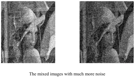
Adding white Gaussian noise to mixed images for three times, the variances of noise are 10, 50 and 100, the noisy mixed images can be depicted by Fig.5.

Λ whitening

∑ ∑

A

s(t) + _x(t)

+

) ( ~_t x

+ _{_}

W

W(0)≠0

∫

×

∑

×

f

g µ

+ _

Learning algorithm

T fg

y(t)

The mixed images with noise once

The mixed images with much noise

The mixed images with much more noise Fig. 5 The noisy mixed images

The separated images by NOISYFASTICA can be depicted by Fig.6.

The separated images by NOISYFASTICA for the first time

The separated images by NOISYFASTICA for the second time

The separated images by NOISYFASTICA for the third time

Fig.6 The separated images by NOISYFASTICA

Using the gradient value as the relaxation factorμ and selecting non-linear functionf

_{( )}

y ₌ y,g( )y =tanh( )y ,

the separated images by the proposed algorithm can be depicted by Fig.7.

The separated images by the proposed algorithm for the second time

The separated images by the proposed algorithm for the third time

Fig.7 The separated images by the proposedalgorithm

We examine the signal-noise ratio of mixing images, noisy mixing images, separation images by NOISYFASTICA and separation images by the proposed algorithm which are shown by Table 1.

TABLE 1

THE SNR COMPARISON OF IMAGES

images

The images SNR with noise once

(dB)

The images SNR with

much noise(dB)

The images SNR with much more

noise(dB)

mixed images

ic -2.3159

lenna 3.2346

noisy mixing images

ic -1.7523 -4.3298 -8.5241

lenna 3.2956 -0.3245 -4.7512

Separation images by

NOISYFASTICA

ic 8.9452 8.7584 8.2568

lenna 11.4687 11.1425 10.8573

separation

ic 9.3652 9.1465 9.0512

lenna 12.3512 11.3578 11.1451

The performance index comparison of NOISYFASTICA and the proposed algorithm can be depicted by Table 2.

TABLE 2

PERFORMANCE INDEX COMPARISON OF NOISYFASTICA AND THE

PROPOSED ALGORITHM

algorithm simulation iteration time（s） PI

NOISYFASTICA

first time 2.6432 0.2987

second time 2.5398 0.3786

third time 2.9568 0.5119

The proposed algorithm

first time 3.7461 0.2376

second time 3.3475 0.3545

third time 3. 4854 0.4435

where performance index

∑

⎥ ⎥ ⎦ ⎤ ⎢

⎢ ⎣ ⎡

⎟ ⎟ ⎠ ⎞ ⎜

⎜ ⎝ ⎛

∑ −

+

⎟ ⎟ ⎠ ⎞ ⎜

⎜ ⎝ ⎛

∑ −

=

= = =

n i

n

k _{j ji}

ki n

k _{j ij}

ik

g g g

g

N 1 1max 1 1max 1

2 1 PI

G is the transmission matrix and it is N×N matrix, and

G=WA,

g

_ij is the element of G, max_jg_ij is the

maximum absolute value of line i, max_j g_ji is the maximum absolute value of row j.

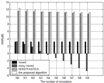
In order to further verify the stability of the proposed algorithm, Adding white Gaussian noise to mixed images for 10 times, the variances of noise are 10, 20,30,40,50,60,70,80,90 , we examine the SNR of mixed images, noisy mixed images, the separation images by NOISYFASTICA and the separation images by the proposed algorithm, the SNR comparison of image ic can be depicted by Fig.7 and the SNR comparison of image lenna can be depicted by Fig.8. where the x axis N0,N1,N2,N3,N4,N5,N6,N7,N8,N9 are the number of the simulations.

Fig.8 The SNR comparison of image lenna

Furtherly, the performance index comparison of NOISYFASTICA and the proposed algorithm for the 10 times simulation can be depicted by Fig.9. The iteration time comparison of NOISYFASTICA and the proposed algorithm can be depicted by Fig.10, where the x axis N0,N1,N2,N3,N4,N5,N6,N7,N8,N9 are the number of the simulations.

Fig.9 The performance index comparison of NOISYFASTICA and the proposed algorithm

Fig.10 The iteration time comparison of NOISYFASTICA and the proposed algorithm

From the simulation results and the data in the table can be seen, with the increase of the noise strength, the antinoise ability of NOISYFASTICA and the proposed algorithm are also very strong even in the case of the images covered by noise, both of them can improve the SNR of the noisy images effectively. Comparing with NOISYFASTICA algorithm, the proposed algorithm has the better performance and separation effect, but the iterative for long time.

V CONCLUSION

1) A method for performing multiple channels blind signal separation in the presence of additive noise is described. The method is proposed of combining neural network and independent component analysis to separate noisy mixed images. The windage wipe off technique was used to correct the infection of noise, a neural network model having denoise capability was adopted to realize the multiple channels blind source separation method for mixing images corrupter with white noise, and a relaxation factor are introduced into the iteration algorithm to improve the convergence.

2) The proposed algorithm reduces the noise influences, overcomes the shortcoming of the traditional ICA cannot be used in the presence of noise model, and makes the online ICA model more easily applied.

3) The simulation and experiment results prove the feasibility and validity of the modeling and control method based on neural network and independent component analysis, which can renew the original image effectively. The results indicate that it has better performances than the classical of NOISYFASTICA and it satisfies the noisy multiple channels blind signal separation problem better. Furthermore, with this algorithm, ICA can be used to solve the problem of more realistic blind signal separation.

ACKNOWLEDGEMENTS

This work was supported by Doctoral Fund of Ministry of Education of China（No. 2011081047）and Shanxi Natural Science Foundation (No. 2013011016-1) and Shanxi Young Science Foundation (No.2013021016-1 ).

REFERENCES

[1] DIAO Guo-ying, HU Gui-jun, LI Gong-yu, CUI

Yun-peng.Application of ICA in the output signal separation of mode group diversity multiplexing system. Journal on Communications,2010,31(9), pp. 118-121.

[2] Huang Qihong,Wang Shuai,Liu zhao．Improved image

feature extraction based on independent component

analysis．Opto-Electronic,2007,34（1）, pp. 123-125

[3] J.F.Cardoso,J.Delabrouille,G.Patanchon ． Independent

component analysis of the cosmic microwave

backgroung．ICA2003,Nara,Japan,2003, pp. 1111~1116

[4] A.Hyvarinen,et al.Imposing sparsity on the mixing matrix

in independent component

[5] J.Anemuller,B.Kollmeier ． Amplitude modulation decorrrelation for convolutive blind source

separation．ICA2000,Helsinki,Finland,2000, pp. 215~220

[6] P.Rajkishore,S.Hiroshi.,S.Kiyohiro．Blind Separation of

Speech by Fixed-Point ICA with Source Adaptive

Negentropy Approximation ． IEICE Trans

Fundamentals,2005,pp. 1683-1692

[7] DIAO Guo-ying, HU Gui-jun, LI Gong-yu, CUI

Yun-peng.Application of ICA in the output signal separation of mode group diversity multiplexing system.

Journal on Communications,2010,31(9), pp. 118-121.

[8] MA Li-yan,LI Hong-wei.An algorithm based on

nonlinear PCA for blind separation of convolutive

mixtures[J]. Journal of Electronics,2008,36(5), pp.

1009-1012.

[9] F.Asano,S.Ikeda,M.Ogawa．Combined approach of

array processing and independent component analysis for

blind separation of acoustic signals．IEEE Transactions

on Speech and Audio Processing,2003,11（3）, pp.

204-215

[10] A.Hyvarinen,E.Oja．A fast fixed-point algorithm for

independent component analysis ． Neural

Computation,1997,9（7）, pp. 1483~1492

[11] A.Hyvarinen．Fast and robust fixed-point algorithms for

independent component analysis．IEEE Trans. Neural

Networks,1999,8（3）, pp. 622~634

[12] P.Rajkishore,S.Hiroshi.,S.Kiyohiro．Blind Separation of

Speech by Fixed-Point ICA with Source Adaptive

Negentropy Approximation ． IEICE Trans

Fundamentals,2005,pp. 1683-1692

[13] LU Feng-bo, HUANG Zhi-tao, JIANG Wen-li. Blind

estimation of spreading sequence of CDMA signals based on Fast-ICA and performance analysis. Journal on Communications,2011,32(8), pp. 136-142

[14] Z.Shi,H.Tang,Y.Tang．A new fixed-point algorithm for

independent component analysis ． Neural

Computing,2004,56, pp. 467-473

[15] A.Hyvarinen．Fast independent component analysis with

noisy data using gaussian moments．In Proc. Int. Symp.

on Circuits and Systems,Orlando,Florida,1999,pp. 57~61

[16] A.Hyvarinen ． Noisy independent component

analysis,maximum likelihood estimation,and competitive

learning．IJCNN,Alaska：1998, pp. 2282~2286

[17] E.Moulines,J.F.Cardoso,E.Gassiat．Maximum likelihood

for blind separation and deconvolution of noisy signals

using mixture modesl．ICASSP,Washington,1998, pp.

3617~3620

[18] A.Hyvarinen．Gaussian moments for noisy independent

component analysis．IEEE Signal Processing,1999,6（6）,

pp. 145~147

[19] Zhang Yinxue and Tian Xuemin. Seismic denoising

based on the modified particle swarm optimization-independent component analysis.Joural of

Oil Geophysical Prosecting, 2012,47(1), pp. 56-62

[20] Hongyan Li, Xueying Zhang. Blind separation of noisy

mixed speech based on independent component analysis and neural network.CMCSN2012, pp. 105-108

[21] Zhou Zhongtan, Dong Guohua, Xu Xin. Independent

component analysis. Beijing:Electronic Industry Press,2007

Hongyan Li was born in Shanxi, China, in 1973, she is an associate professor at Taiyuan University of Technology. Since 2009, she has been a ph.D.degree candidate in circuit and system from Taiyuan University of Technology. She is cerrently pursuing the postdoctoral at Taiyuan University of Technology.Her research interests includes blind signal processing and pattern identification.

Xueying Zhang was born in Shanxi, China, in 1964, she received the ph.D.degree in underwater acoustic engineering from harbin engineering university. Since 1999, she has been a professor at Taiyuan University of Technology. Her research

interests includes speech signal processing, multimedia

communication, embedded system and application and the