Probability Hypothesis Density Filter Based on
Gaussian-Hermite Numerical Integration
Jinguang Chen
School of Computer Science, Xi’an Polytechnic University, Xi’an 710048, China School of Electronic Engineering, Xidian University, Xi’an 710071, China
Email: [email protected]
Ni Wang, Lili Ma, Tiantian Zhao
School of Computer Science, Xi’an Polytechnic University, Xi’an 710048, China Email: [email protected]
Abstract—This work addresses the multi-target tracking
problem in the nonlinear Gaussian system. One probability hypothesis density filtering algorithm based on Gaussian-Hermite numerical integration is proposed. In order to calculate integrations in the Gaussian mixture probability hypothesis density filter, the Gaussian-Hermite numerical integration method is used to approximate the integration. In the filtering stages of prediction and update, we calculate the corresponding Gaussian-Hermite integral points and weights, employ the method of numerical accumulation to approximate the integrations of the Gaussian mixture probability hypothesis density filter. Then the corresponding Gaussian items are calculated and the recursions of Gaussian mixture are implemented. The new algorithm can estimate not only the state vector effectively but also the number of targets accurately. Moreover, its time complexity increases in a low level. The simulation results show that the new algorithm can improve the accuracy of target tracking, and its time complexity keeps the same order of magnitude as the extended Kalman Gaussian mixture probability hypothesis density filter.
Index Terms—probability hypothesis density filter, random
finite sets, Gaussian-Hermite numerical integration, multi-target tracking, state estimation
I. INTRODUCTION
In recent years, the theory of random finite sets (RFS) is widely used in the fields of information fusion which is dealing with point estimation [1] and target
tracking. More and more scholars pay attention to this theory. Random sets theory mainly refers to the random finite sets theory, it can solve the problem of multi-target tracking effectively under a complex environment. It already becomes one of the most popular direction in the multi-target tracking research field [2]. Mahler's
probability hypothesis density (PHD) filter [3] is a filtering
method based on the framework of RFS. This method
represents multi-target state and measurement as random finite sets, and adopts an approach which is similar to the Bayesian theory to implement in a unified style. The complexity of the data association problem is avoided in this progress. Because formulas of the PHD filtering recursion contain integrals, it is generally difficult to obtain the analytical solution. To solve this problem, Vo et al. propose the Gaussian mixture PHD (GM-PHD) filter [4] which is applicable to the linear Gaussian systems.
This algorithm assumes that the multi-target PHD could be written as the form of Gaussian mixture, then at each time step, the prediction and update PHD can also subject to the distribution of Gaussian mixture. Thus the recursive Gaussian mixture PHD filter algorithm is derived. Furthermore, Clark et al. prove that the GM-PHD filter is convergence, and present the error boundary in trim and merge phases [5]. For multi-target tracking
problems with nonlinear Gaussian assumption, the extended Kalman PHD (EK-PHD) filtering algorithm is given in [4]. EK-PHD uses the method of Taylor series expansion to get the local linearization of nonlinear functions, and then the GM-PHD is employed directly. However, only under the condition of weak nonlinear system, the EK-PHD can get satisfied filtering accuracy. If system is strong nonlinear, due to the large linear truncation errors, the filtering accuracy become low. In order to improve the accuracy in the strong nonlinear system, article [6] which is based on particle filter [7]
presents the particle PHD (P-PHD) filter, also known as sequential Monte Carlo PHD (SMC-PHD). The algorithm uses a large number of particles and weights to approximate the nonlinear transformation of random variables. It can obtain higher filtering accuracy and can also apply to the condition of the system which is nonlinear and non-Gaussian. Then the convergence of P-PHD is analyzed and proved in [8], and the boundary of the mean square error (MSE) is derived. Literature [9] adopts unscented particle filter (UPF) to implement P-PHD filter, which uses unscented Kalman filter to get better importance density function and sample particles from it. In this way, good error performance is acquired. However, time complexity of this algorithm is very high Manuscript received on September 7, 2013.
and real-time performance in filtering stage is poor. So, people try to find some other PHD filters whose complexities are not so high. Such as the unscented Kalman PHD (UK-PHD)[4] filter with nonlinear Gaussian
assumption, which uses unscented transform to determine the sampling points to characterize the statistical properties of Gaussian random vector, and approximates the state of the system’s posterior probability. In [10], the central difference Kalman (CDK) filter is combined with PHD, and the CDK-PHD filter is proposed. This method uses the Stirling interpolation formula to approximate the polynomial of nonlinear function. It improves the estimation accuracy. Cubature Kalman Filter (CKF) [11]
can be combined with the PHD, and the cubature PHD filter is given in [12]. This algorithm adopts the sampling rules of third-order spherical cubature-radial to compute the probability distribution of target state, which solves the computing problems of nonlinear state equation and observation equation.
As the Gaussian-Hermite numerical integration is applied to the nonlinear Gaussian filtering system, it is the Gaussian-sum quadrature Kalman (QKF) filter [13].
Under the inspiration of the work above, we apply the Gaussian-Hermite numerical integration method to the PHD filter process, and obtain a new PHD filter which can deal with multi-target nonlinear tracking system, namely the Gaussian-Hermite probability hypothesis density filter (GH-PHD). Compared with the EK-PHD filter algorithm, new algorithm improves the filtering accuracy. Although time complexity of this algorithm increases, it keeps the same order of magnitude with EK-PHD filter algorithm. So, it is acceptable in many practical applications.
II. PROBLEM FORMULATION
In the process of multi-target tracking, old targets may be disappearing and new targets may be appearing in one time step so that the number of targets is changing over time. Suppose the number of targets is M k( ) at timek,
by using the random finite sets, the state set of targets can be represented as Xk ={ ,xk,1 xk M k, ( )} and the
measurement set can be represented as
,1 , ( )
{ , }
k = k k N k
Z z z , where N k( ) is the measurement number at time k.
Suppose that the state set is Xk at timek, then at time 1
k+ the state set of targets can be expressed as
1 1 ( ) 1 ( ) 1
k+ =Sk+k k Bk+k k Γk+
X X ∪ X ∪ (1)
where Sk+1k( )Xk is the RFS of targets survival,
1 ( )k
k k
B+ X is the RFS of targets spawned at time k+1
from previous targets with stateXk, Γk+1is the RFS of
spontaneous birth at time k+1 . Usually we use
1
( k k)
f X+ X to express the transition density of
multi-target state.
Similarly, at time k the set of measurements can be
expressed as
( ) k = k Θk k
Z K ∪ X (2)
where Kk is the measurement random set of false measurements or clutter. Θk(Xk) is the measurement random set produced by the real targets. Usually we use
( k k)
g Z X to express the measurement likelihood
function.
In the target tracking system, it is usually assumed that the dynamic model and measurement model of a single target are represented as follows
1
( ) k = f k− + k
x x ω (3) ( )
k =h k + k
z x υ (4) where ωk and υk are both the additive Gaussian noises.
k
x is the state vector, f( )⋅ and h( )⋅ are the transition
function and the measurement function, respectively. Assume p( )x0 is the initial state distribution, the
purpose of target tracking is to estimate the posterior distribution recursively, thus to estimate the target state and the target number.
III. GAUSSIAN-HERMITE NUMERICAL INTEGRATION Gaussian-Hermite filter is a nonlinear Bayes filter under the assumption of Gaussian distribution. It is a kind of recursive filtering method based on Gaussian-Hermite numerical integration [13], which is implemented by
choosing integral points and the corresponding weights to enhance the accuracy of the system state mean and the variance estimate [14].
Assume that g x( ) is a weighted integral function on an interval ( , )a b , then the integral can be expressed as
( ) ab ( ) ( )
I g =
∫
W x g x dx (5)where W x( ) is a weighted function. If we use m
numerical points to integrate, formula (5) can be approximated as
1
( ) m i ( )i i
I g w gξ
=
≈
∑
(6)where ξi is the standard integral point, wi is its corresponding weight.
Firstly, we consider one-dimensional situation, it is assumed that a random variable x with a Gaussian
probability density is p x( )=N( ;0,1)x . The expectation of
the function g x( ) can be approximated as
1
[ ( )] ( )N( ;0,1)
( ) R
m l l l
g x g x x dx
w g ξ =
Ε =
≈
∫
tridiagonal matrix with zero diagonal elements and other elements are
, 1 2,1 ( 1)
i i
J + = i ≤ ≤i m− (8)
Here, m is the number of standard integral points. In fact,
the specific number of integral points is determined by m
and the dimension of state vector. For example, if m=5, then the dimension of state vector is 4, it will have 625 points. If m>3, through experiments we found that the filtering precision of algorithm improvement is not big, but its time complexity increases significantly. For these reasons, we select m=3 in the experiment. The standard integral point is taken to be ξl= 2εl, where εl is the l -th eigenvalue of matrix J; the corresponding weight is
2 1
( ) l l
w = ν , where ( )νl 1 is the first element of the l-th
normalized eigenvector of matrix J.
Furthermore, we can extend one dimensional case to multi-dimensional case. Assume a random vector x has
a Gaussian density ( ) N( ; , )p x = x0 Inx , where Inx is the identity matrix with nx×nx dimensions. Since each element of x is mutually uncorrelated, integral rule of
x
n dimensions Gaussian-Hermite is as follows:
1 1 1
1 1
1
[ ( )] ( )N( ; , )
... ( ... )
( ).
nx nx
nx nx R
m m
l l l l
l l
m l l l
g g d
w w g
w g
ξ ξ
= =
=
Ε =
≈
=
∫
∑
∑
∑
x x x I x
ξ
0
(9)
where 1 T
1
[ ... ] , x
nx j
n l = ξ ξl l wl =
∏
j=wlξ .
Moreover, we further assume that a random vector x
has a Gaussian density p( ) N( ; , )x = x x Pˆ , do Cholesky decomposition of P, and get P =SST, y=S−1(x x− ˆ),
then
1 1 1
T
1 1
1
1
ˆ E[ ( )] ( )N( ; , )
ˆ
( )N( ; , )
ˆ ... ( [ ... ] )
ˆ
( )
( ).
x
nx nx
nx nx
nx
n
m m
l l l l
l l
m
l l l
m l l l
g g d
g d
w w g
w g
w g
ξ ξ
ξ
= =
=
= =
= +
≈ +
= +
=
∫
∫
∑
∑
∑
∑
x x x x P x
Sy x y I y
S x
S x
x
0
(10)
Now, integral points can be obtained by ˆ l = ξl +
x S x (11)
IV. PROBABILITY HYPOTHESIS DENSITY FILTER Traditional multi-target tracking algorithms are related to data association, which means we need to determine the corresponding relationship between tracks and measurements. The computational complexity of data association grows exponentially along with the increase
of the number of targets and measurements. Mahler's PHD filter is a kind of target tracking algorithm based on random sets theory [3]. This algorithm can avoid the
complex progress of data association and can deal with multi-target tracking problem in an effective manner. The traditional Bayes filter propagates global probability density, but the calculation of global probability density in multi-target tracking is very difficult. Aiming at this problem, PHD propagates first-order statistics of the random finite sets via the posterior probability density. Also because of PHD propagation is posterior intensity of the state space, its integral in any state space is the expectation of targets’ number. Therefore, PHD filter can not only track the multi-target state when target number is unknown or changing over time, but also estimate the target number. Similar to the Bayes filter in multi-target tracking, the recursions in PHD filter also include prediction stage and update stage.
At time k, the PHD prediction formula is
1: 1 , 1 1
1 1
1 1 1 1: 1 1
1
( ) ( ) [ ( ) ( )
( )] ( )
k k k k S k k k k
k k k k
k k k k k k
k k
D p f
D d
γ β
− − −
− −
− − − − −
−
= +
+
∫
x Z x x x x
x x x Z x
(12) where γk( )xk is intensity of the spontaneous birth RFS at time k , βk k−1(x xk k−1) is intensity of the RFS
spawned at time k by a target with previous state xk−1,
, ( 1)
S k k
p x − is the probability that a target with previous
state xk−1 still exists at time k . fk k−1(x xk k−1) is the
transition probability density of target state.
1 1: 1
1( k k )
k k
D − x − Z − is the posterior intensity of target at
time k−1.
The integral of PHD prediction function Dk k−1( )⋅ is the
estimation of target number, i.e.,
1: 1
1 1( ) 1 1 1
S B
k k k
k k k k k k k k k k
N − =
∫
D − x Z − dx =NΓ − +N − +N − (13)where
1 k( )k k
k k
NΓ − =
∫
γ x dx (14), 1 1 1 1 1: 1 1
1 ( ) 1( ) ( )
S
S k k k k k k k k
k k k k
N − =
∫
p x − f − x x − D− x − Z − dx −(15)
1 1 1 1: 1
1 1( ) ( )
B
k k k k k k
k k k k
N − =
∫
β − x x − D− x − Z − dx (16)Here, formulas (14)-(16) express the expectation of spontaneous birth target number, the expectation of survival target number, and the expectation of spawned target number, respectively.
At time k, the PHD update formula is
1: , 1 1: 1
, 1 1: 1
, 1 1: 1
( ) (1 ( )) ( )
( ) ( ) ( )
( ) ( ) ( ) ( )
k k
k k k D k k k k k k D k k k k k k k k k
k D k k k k k k k k k k
D p D
p g D
p g D d
κ
− −
− −
∈ − −
= − +
+
∑
∫
z Zx Z x x Z
x z x x Z
z x z x x Z x
where κk( )z =λkc zk( ) is the intensity of clutter RFS at time k, c zk( ) is probability density of clutter, λk is the
average number of clutter. Assume that the number of clutter which appears at each time obeys Poisson distribution, gk(z xk k) is the measurement likelihood function of target, pD k, ( )xk is the detection probability.
Similarly, the update formula of the expectation value of the target number is
1:
, 1: 1
1 1
, 1 1: 1
, 1 1: 1
( )
( ) ( )
( ) ( ) ( )
( ) ( ) ( ) ( )
k
k k k k k
D k k k k k
k k k k
D k k k k k k k k k k k D k k k k k k k k k k
N D d
N p D d
p g D d
p g D d
κ − − − − − ∈ − − = = − + +
∫
∫
∫
∑
∫
z Zx Z x
x x Z x
x z x x Z x
z x z x x Z x
(18) From the prediction equation (12) and update equation (17) above, there are integrals among them. These integrations have no analytical solution in generally. In fact, the integral form can be written as an integral form of a nonlinear function multiplied by a Gaussian distribution, i.e.,
nonlinear function * Gaussian distributiond
∫
x (19)This kind of integral form can be approximated by using the method of formula (10), thus gaining a Gaussian-Hermite PHD filter algorithm.
V. GAUSSIAN-HERMITE PHDFILTER
Assume that the collection for Gaussian mixture components is ( ) ( ) ( ) 1
1 1 1 1
{ i , i , i}Jk
k k k i
w −
− m− P− = at time k−1, and at
time k the measurement set is
Z
k. For birth targets, theprediction stage is the same as that of the GM-PHD filter in which the numerical integrations are not needed. For survival targets, it uses numerical integration in recursions. In time update stage, for the variance of every Gaussian items, do Cholesky decomposition, i.e.,
( ) ( ) ( ) T
1 1( 1)
i i i
k− = k− k−
P S S (20) Then, use formula (10) to calculate the integral points of each Gaussian component
( ) ( ) ( )
, 1i i1 i1
l k− = k−ξl+ k−
x S m (21) Next, predict each integral point according to the state transition equation
( ) ( )
, 1
, 1 ( )
i i
l k l k k− = f −
x x (22) Finally, one-step prediction mean and variance of survival targets are given as
( ) ( )
1 , 1
1
m
i i
l k k l k k
l
w
− −
=
=
∑
m x (23)
( ) ( ) ( ) T ( ) ( ) T
1 , 1 , 1 1 1
1
ˆ ˆ
( ) ( )
m
i i i i i
l k
k k l k k l k k k k k k l
w
− − − − −
=
=
∑
− +P x x x x Q (24)
where wl is the corresponding weight of Gaussian-Hermite integral point and Qk is the variance of process noise.
Assume that the prediction result of the component collection for Gaussian Mixture is ( ) ( ) ( ) 1
1
1 1 1
{ i , i , i }Jk k i k k k k k k
w −
=
− m − P − ,
in the measurement update, we do Cholesky decomposition for ( )
1
i k k−
P as well as formula (20), i.e.,
( ) ( ) ( ) T
1 1( 1)
i i i
k k− = k k− k k−
P S S , then the new integral point is
( ) ( ) ( )
, 1 1 1
i i i
l l k k− = k k−ξ + k k−
x S m (25) Then, calculate integral point of measurement prediction
( ) ( )
1 , 1
1
( )
m
i i
l k k l k k
l
w h
− −
=
=
∑
z x (26)
Next, state update and covariance update of the integral point are calculated as
( ) ( ) ( ) ( ) ( )
1 ( 1)
i i i i i
k = k k− + k − k k−
x m K z z (27)
( ) ( ) ( ) ( ) ( ) T
1 ( )
i i i i i
k = k k− − k zz k
P P Κ P Κ (28)
where h( )⋅ is the measurement function of target, z( )i is the actual measurement value of the corresponding time,
( )i k
Κ is the filter gain, it is calculated as follows:
( )i ( )i ( ( )i ) 1
k
−
= xz zz
Κ P P (29)
( ) ( ) ( ) T ( ) ( ) T
, 1 , 1 1 1
1
( ) ( )
m
i i i i i
zz k l l k k l k k k k k k l
w − − − −
=
= +
∑
−P R z z z z (30)
( ) ( ) ( ) T ( ) ( ) T
, 1 , 1 1 1
1
( ) ( )
m
i i i i i
xz l l k k l k k k k k k l
w − − − −
=
=
∑
−P x z m z (31)
where ( ) ( )
, 1 ( , 1)
i i
l k k− =h l k k−
z x .
From the description above, the pseudo code for the GH-PHD filter is summarized as below:
Step 1: prediction for spontaneous birth targets 0
i=
for j=1, ,Jγ,k : 1
i = +i
( ) ( )
, 1
i j
k k k− = γ
m m , ( )i 1 ( ),j k k k
w − =wγ , ( )i 1 ( ),j
k k k− = γ
P P
end
Step 2: prediction for existing targets
( ) ( ) ( ) T
1 1( 1)
j j j
k− = k− k−
P S S
for j=1,...,Jk−1
: 1
i = +i
for l=1, ,m
( ) ( ) ( )
, 1i j1 j1
l k− = k−ξl+ k−
x S m
( ) ( )
, 1 ( , 1)
i i
l k k− = f l k k−
x x end ( ) ( ) , 1 1 i j
S k k k k
w − = p w− , ( ) 1 ( ), 1
1
m
i i
l k k l k k
l w − − = =
∑
m x( ) ( ) ( ) T ( ) ( ) T
1 , 1 , 1 1 1
1
( ) ( )
m
i i i i i
l k
k k l k k l k k k k k k l
w
− − − − −
=
=
∑
− +end
1
k k
J − =i
Step 3: each component in the measurement update for j=1,...,Jk k−1
( ) ( )
1 , 1
1
ˆ j m j
l k k l k k
l
w
− −
=
=
∑
z z
( ) ( ) T ( ) ( ) T
, 1 , 1 1 1
1
ˆ ˆ
( ) ( )
m
j j j j
k l l k k l k k k k k k l
w − − − −
=
= +
∑
−zz
P R z z z z
( ) T ( ) ( ) T
, 1 , 1 1 1
1
ˆ
( ) ( )
m
j j j
l l k k l k k k k k k l
w − − − −
=
=
∑
−xz
P x z m z
( )j 1
k
− = xz zz
Κ P P , ( )j ( )j 1 ( )j ( ( ) Tj )
k k
k k = k k− − zz
P P Κ P Κ
end
Step 4: measurement update for j=1,...,Jk k−1
( ) ( )
, 1
(1 )
j j
k D k k k
w = −p w −
( ) ( ) ( ) ( )
1, 1
j j j j
k = k k− k = k k−
m m P P
end : 0
i =
for z Z∈ k
: 1
i = +i
for j=1,...,Jk k−1
( ) ( ) ( ) T
1 1( 1)
i i i
k k− = k k− k k−
P S S
for l=1, m
( ) ( ) ( )
,i 1 i 1 l i 1
l k k− = k k−ξ + k k−
x S m
( ) ( )
, 1 ( , 1)
i i
l k k− =h l k k−
z x
end
( ) ( ) ( ) ( )
, 1N( ;ˆ 1, )
i j j j
k D k k k k k
w = p w − z z − Pzz ,
( ) ( ) ( ) ( ) ( )
1 ( ˆ 1)
i j j j j
k = k k− + k − k k−
m m K z z
( )i ( )j k = k k
P P
end
1
( ) ( )
1 ( )
1
, 1,..., ( ) k k
j
i k
k J i k k
k i k
w
w j J
w
κ − −
=
= =
+
∑
z
end
1 1
k k k k k
J =iJ − +J −
Output: ( ) ( ) ( ) 1
{ i , i , i}Jk k k k i
w m P = .
The number of Gaussian items for the posterior probability density will be increasing as time passing. As a result, a large number of calculation time is wasted to update the Gaussian items which have small weights. In order to control the number of Gaussian items, we can
use pruning and merging method which is described in [4]. This can be done by setting a truncation threshold T and a merging threshold U . In pruning stage, Some
Gaussian items are abandoned as their weights are smaller than truncation threshold. As a result, the Gaussian items whose weights are greater than truncation threshold are kept. In merging stage, give two Gaussian items { ,( )i ( )i, ( )i}
k k k
w m P and { ( )j, ( )j, ( )j}
k k k
w m P , when the
means and variances of the two Gaussian items meet
( ) ( ) T ( ) 1 ( ) ( )
( i j) ( i) ( i j)
k k k k k U
−
− − ≤
m m P m m , the two Gaussian
items will be merged.
For multi-target state extraction, the clustering method is commonly used in the P-PHD filter[15]. Under the
condition of Gaussian mixture, we generally use the method mentioned in [4] to extract targets’ state. Given a threshold, the Gaussian component with weight which is greater than the threshold can be regarded as a target and the corresponding state is the estimation of the target.
VI. SIMULATION EXPERIMENT AND RESULT ANALYSIS In the simulation region, assume that there are two targets. Each target is moving via constant velocity model or constant turn model. Target 1 appears at time k=1, and dies at time k=40; target 2 appears at time k=6,
and dies at time k=49 . Two targets both travel in straight lines before time k=16, then they are making turns until time k=34, and the targets resume straight trajectories after time k=34.
The state vector of targets is [ ]T
k = x x y y
x , it
consists of position component ( , )x y and velocity
component
( , )
x y
. Each target has survival probability, 0.99
S k
p = and detection probability pD k, =0.98 . The
corresponding motion equation is
1
k = k− + k
x Fx Gω (32) where transition matrix of state noise is
T 2
2
2 0 0
0 0 2
T T
T T
⎡ ⎤
=⎢ ⎥
⎣ ⎦
G . When targets do constant
velocity motion, blkdiag 1 , 1 0
0 1 0 1
T
⎛⎡ ⎤ ⎡ ⎤⎞
= ⎜⎢ ⎥ ⎢ ⎥⎟
⎣ ⎦ ⎣ ⎦
⎝ ⎠
F ; when
targets do constant turn motion,
sin 1 cos
1 0
0 cos 0 sin
1 cos sin
0 1
0 sin 0 cos
T T
T T
T T
T T
Ω − Ω
⎡ − ⎤
⎢ Ω Ω ⎥
⎢ ⎥
Ω − Ω
⎢ ⎥
=⎢ ⎥
− Ω Ω
⎢ ⎥
Ω Ω
⎢ ⎥
⎢ Ω Ω ⎥
⎣ ⎦
F . ωk is white
Gaussian noise, state noise matrix is diag([0.5 0.5])
k =
Q , sampling period is T=1s, and
the turn rate is Ω = π(5 80)rad/s.
2 2
arctan( ) k
k k
k
y x r
x y
θ ⎡ ⎤
⎡ ⎤ ⎢ ⎥
=⎢ ⎥ ⎢= ⎥+
⎣ ⎦ ⎢⎣ + ⎥⎦
z υ (33)
where υk ~ N( ; , )⋅0 Rk , and
2 2
diag([ k k]) k = σθ σr
R ,
2 ( 180) k
θ
σ = × π rad/s, 8σ =rk m. Measurement vector
k
z includes two components, the bearing θk and range rk. For convenience, assume that there are no spawned targets. And suppose PHD of spontaneous birth target random sets is
(1) (2)
( ) 0.1N( ; , ) 0.1N( ; , )
k γ γ γ γ
γ
x = x m P + x m Pwhere
[
]
T(1) -1000 60 500 0
γ =
m ,
[
]
T(2) 1050 -62 1070 0
γ =
m ,
diag([100 40 100 40])
γ =
P . Clutter is uniformly
distributed in the surveillance region, and the number of clutter subjects to a Poisson distribution whose mean is
5
r= . Pruning threshold is Tprun= −1e 5 , merging
threshold is Uprun =4. cospa =70 is the adjustment factor
of state error and cardinality error, pospa =2 is the
distance of OSPA, Jmax=100 is the largest number of
Gaussian components. The entire time of the simulation
is 49 s, the surveillance region is
[−π2, 2]rad [0,1600]mπ × .
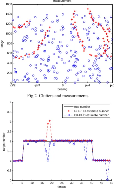
Results of the GH-PHD filter and the EK-PHD filter are shown in Fig 1. From Fig 1, we are easily known that EK-PHD filter and GH-PHD filter both have better estimate of targets. The difference is that the tracking performance of GH-PHD filter is better than that of EK-PHD. EK-PHD filter cannot accurately estimate the location of targets, it will also leak with some targets in the turn stage, and GH-PHD filter can accurately estimate the location of targets. Target trajectories and measurements in the area of the surveillance are shown in Fig 2. The marks of blue “ ο ” express the clutter distribution, the marks of red “*” are the true trajectory of targets. r=5 is the number of clutter and it subjects to the Poisson distribution, the clutter uniformly distributes in the whole surveillance area.
-1000 -500 0 500 1000 1500 400
500 600 700 800 900 1000 1100 1200
target trajectory
x position
y
p
o
s
itio
n true trajectory
GH-PHD estimate EK-PHD estimate
Fig 1 The position of targets estimated via GH-PHD filter and EK-PHD filter
Fig 3 displays the true number and the estimation number of targets of GH-PHD filter and EK-PHD filter throughout the simulation by time step. From Fig 3, we know that target number estimated by GH-PHD algorithm matched with the true target number well. It appears that the deviation of estimation only happened at time k=18 and k=19, at other time it can accurately
estimate the number of targets; but the target number which is estimated by EK-PHD filter algorithm and the true target number have a few differences.
-pi/20 -pi/4 0 pi/4 pi/2
200 400 600 800 1000 1200 1400 1600
bearing
range
measurement
Fig 2 Clutters and measurements
0 5 10 15 20 25 30 35 40 45 50 0
0.5 1 1.5 2 2.5 3 3.5 4
time/s
tar
g
et
num
ber
true number GH-PHD estimate number EK-PHD estimate number
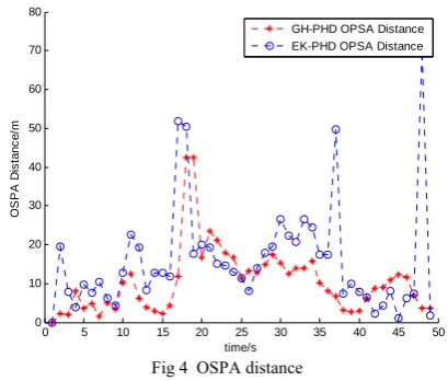
Fig 3 The true number and the estimation number of targets In order to evaluate the accuracy of multi-target tracking filter, optimal subpattern assignment distance (OSPA)[16] is used, which can measure the difference
between sets well, and it is one of the most popular evaluation criteria which has been used by many scholars in recent years. OSPA distance in the simulation is displayed in Fig 4. We are easy to know that the OSPA of GH-PHD filter is smaller than that of EK-PHD, although a few steps’ OSPA is high, like the case at timek=18, however, the performance is better than EK-PHD’s as a whole.
consumes 10.0900 seconds and EK-PHD filter consumes 0.9521 seconds.
0 5 10 15 20 25 30 35 40 45 50 0
10 20 30 40 50 60 70 80
time/s
O
S
P
A
D
ist
a
n
ce
/m
GH-PHD OPSA Distance EK-PHD OPSA Distance
Fig 4 OSPA distance VII. CONCLUSION
Aiming at the probability hypothesis density filter based on the theory of random finite sets in the multi-target tracking problem, this paper combines Gaussian-Hermite numerical integral with Gaussian mixture PHD filter, and one algorithm to deal with nonlinear Gaussian system is presented, i.e., GH-PHD filter. In this approach, the joint distribution of targets and the number of targets can be well estimated, even if the target number is unknown or changing with time. It has good satisfied accuracy in multi-target tracking system. The proposed algorithm is suitable for the nonlinear clutter environment, and it breaks through the limitation of GM-PHD which is only suitable for linear system. For solving the multi-target tracking under a nonlinear system, the new algorithm provides a new implemented approach. The new algorithm calculates the integral points and weights of every Gaussian items in PHD recursion so that the computation of new algorithm is larger than that of EK-PHD filter. But the computational complexity still keeps in the same order of magnitude, so it is acceptable in many engineering applications.
ACKNOWLEDGMENT
This work was supported by the National Natural Science Foundation of China (61201118), the China Postdoctoral Science Foundation (2013M532020), the Scientific Research Program Funded by Shaanxi Provincial Education Department (12JK0529), and the National Training Programs of Innovation and Entrepreneurship for Undergraduates (201310709006).
REFERENCES
[1] Xintao Xia, Leilei Gao, Jianfeng Chen, “Fusion method for true value estimation based on information poor theory”, Journal of Software, 7(5), pp. 1014-1021, 2012.
[2] Mahler R.P.S, “Statistical Multisource Multitarget Information Fusion”, Artech House Publishers, 2007. [3] Mahler R.P.S, “Multitarget Bayes filtering via first-order
multitarget moments”, IEEE Transactions on Aerospace and Electronic Systems, 39(4), pp. 1152-1178, 2003.
[4] Ba-Ngu Vo, Wing-Kin Ma, “The Gaussian mixture probability hypothesis density filter”, IEEE Transactions on Signal Processing, 54(11), pp. 4091-4104, 2006. [5] Clark D, Ba-Ngu Vo, “Convergence analysis of the
Gaussian mixture PHD filter”, IEEE Transactions on Signal Processing, 55(4), pp. 1204-1212, 2007.
[6] Ba-Ngu Vo, Singh S, Doucet A, “Sequential Monte Carlo methods for multi-target filtering with random finite sets”, IEEE Transactions on Aerospace and Electronic Systems, 41(4), pp. 1224-1245, 2005.
[7] Junying Meng, Jiaomin Liu, Juan Wang, et al, “Target tracking based on optimized particle filter algorithm”, Journal of Software, 8(5), pp. 1140-1144, 2013.
[8] Daniel Edward Clark, Judith Bell, “Convergence results for the particle PHD filter”, IEEE Transactions on Signal Processing, 54(7), pp. 2652-2661, 2006.
[9] Fan-bin Meng, Yan-ling Hao, Chong-meng Zhang, et al, “Sequential fusion algorithm based on unscented particle probability hypothesis density filter”, Systems Engineering and Electronics, 33(1), pp. 30-34, 2011 (in Chinese). [10]Li-ming Chen, Zhe Chen, Fu-liang Yin, et al, “Central
difference Kalman-probability hypothesis density filter for multi-target tracking”, Control and Decision, 28(1), pp. 36-42+48, 2013 (in Chinese).
[11]Arasaratnam I, Haykin S, “Cubature Kalman filters”, IEEE Transactions on Automatic Control, 54(6), pp. 1254-1269, 2009.
[12]Pin Wang, Wei-xin Xie, Zong-xiang Liu, et al, “A novel Gaussian Mixture PHD filter for nonlinear models”, Acta Electronica Sinica, 40(8), pp. 1597-1602, 2012 (in Chinese).
[13]Arasaratnam I, Haykin S, “Discrete-time nonlinear filtering algorithms using Gauss-Hermite quadrature”, Proceedings of the IEEE, 95(5), pp. 953-977, 2007.
[14]Challa S, Bar-Shalom Y, Krishnamurthy V, “Nonlinear filtering via generalized edgeworth series and Gauss– Hermite quadrature”, IEEE Transactions on Signal Processing, 48(6), pp. 1816-1820, 2000.
[15]Weifeng Liu, Chongzhao Han, Feng Lian, et al, “Multitarget state extraction for the PHD filter using MCMC approach”, IEEE Transactions on Aerospace and Electronic Systems, 46(2), pp. 864-883, 2010.
[16]Schuhmacher D, Ba-Tuong Vo, Ba-Ngu Vo, “A consistent metric for performance evaluation of multi-object filters”, IEEE Transactions on Signal Processing, 56(8), pp. 3447-3457, 2008.
Dr. Jinguang Chen (1977-): He was born in Henan Province,