Quantifying space, understanding minds: A visual summary approach

REVIEWARTICLE

Quantifying space, understanding

minds: A visual summary approach

Mark Simpson

, Kai-Florian Richter

, Jan Oliver Wallgrün

,

and Alexander Klippel

1

The Department of Geography, The Pennsylvania State University, PA, USA.

2_{Department of Geography, University of Zurich, Zurich, Switzerland.}

Received: July 7, 2016; returned: September 14, 2016; revised: January 1, 2017; accepted: February 25, 2017.

Abstract:This paper presents an illustrated, validated taxonomy of research that compares spatial measures to human behavior. Spatial measures quantify the spatial characteristics of environments, such as the centrality of intersections in a street network or the accessi-bility of a room in a building from all the other rooms. While spatial measures have been of interest to spatial sciences, they are also of importance in the behavioral sciences for use in modeling human behavior. A high correlation between values for spatial measures and specific behaviors can provide insights into an environment’s legibility, and contribute to a deeper understanding of human spatial cognition. Research in this area takes place in sev-eral domains, which makes a full understanding of existing literature difficult. To address this challenge, we adopt a visual summary approach. Literature is analyzed, and recurring topics are identified and validated with independent inter-rater agreement tasks in order to create a robust taxonomy for spatial measures and human behavior. The taxonomy is then illustrated with a visual representation that allows for at-a-glance visual access to the content of individual research papers in a corpus. A public web interface has been created that allows interested researchers to add to the database and create visual summaries for their research papers using our taxonomy.

Keywords:space syntax, spatial measures, environmental cognition, visual summaries

1

Introduction

characteristics and behavior has been well established, but most findings rely on qualita-tive descriptors that make comparing findings difficult [65]. Comparing behavior to spa-tial characteristics more systematically requires the formalization of those characteristics, which we refer to here asspatial measures. Broadly, spatial measures are techniques and methods for quantitatively measuring space and spatial relationships. Importantly, they can move beyond classical metric understanding (e.g., distance and direction) and mea-sure aspects such as relative centrality. They arise in several areas of research, perhaps most prominently within the realm ofspace syntax[27]. They allow for different environments to be directly compared in terms of their spatial characteristics, and to quantitatively compare those characteristics to various spatial behavioral measures (e.g., wayfinding performance). The primary motivation for understanding the relationship between spatial measures and human behavior is to gain insight into the underlying mental processes that drive hu-man behavior in space. Spatial measures can also be used as behavioral models directly (i.e., to predict behavior in an environment) in fields such as architecture and urban plan-ning [16,24]. Understanding how spatial characteristics of an environment may influence human behavior is of wider importance because it can provide insights into how to com-pensate for difficulties in understanding an environment, such as during wayfinding, and into how to create spaces that are more easily navigable. Almost everyone has become lost in a confusing building at one time or another, and some places seem difficult to navigate even if one has been there many times before [11]. What may be a mere inconvenience in normal activity may become critical in emergency situations.

Despite the importance of this research domain, an overview of existing research to help synthesize knowledge across disciplinary boundaries is missing (see Bafna [2], Carlson et al. [11], and Dalton et al. [15] for existing reviews in the area). We use the visual summary approach, adapted from Mason et al. [41] to create an illustrated taxonomy that is intended to enable such an overview. This method involves the manual review of selected literature to construct taxonomic categories, which are represented in a diagram called a visual sum-mary. Literature is selected according to its relevance as judged by the authors, with the intention of capturing the breadth of the target research area. Once a paper is classified, a visual summary can be made to show which categories it contains. A series of visual sum-maries then allows a user to quickly compare a series of papers according to their content (see Figure5for an example). We have implemented a web interface which allows authors (or other interested parties) to classify literature and create visual summaries themselves, which consequently will grow the database of classified literature and, over time, will allow for increasingly detailed analyses.

2

Background

In this section, we will review key trends in environmental cognition and spatial measures research in order to provide some context to the taxonomy and visual summary we have created. This section is kept deliberately short, as a significant amount of research is re-viewed in the course of explaining the taxonomy itself, in Section4.1.

2.1

Environmental cognition and spatial measures

A fundamental challenge in this area of research is that human spatial memory structures are distorted, and that the degree and type of distortion can vary with the spatial properties of an environment [17,67]. Following Golledge [22], we refer to these spatial memory struc-tures asinternal representations. Since the biological basis for spatial information storage is not thoroughly understood in humans, “internal representations must be inferred from one or more external symbolic representations (e.g., sketch maps of a city) or from some other forms of observable behavior (e.g., search behavior to find a specific location)” [22]. Direct observation of internal representations is currently not possible, so researchers must instead examine behaviors which make use of them.

Spatial measures allow for more objective connections between spatial behavior and the spatial aspects of the environment. The basic premise is: if a measure correlates well with some spatial behavior within an environment, there must be some connection be-tween how the measure represents (or operates on) that environment and how the human brain does. However, this relationship is not easy to establish. There are many potential stimuli involved in creating environmental knowledge, and individual strategies for activ-ities such as wayfinding differ considerably [66]. This indicates that it may be necessary to combine different measures to capture the variety and combinations of spatial aspects used by humans in order to fully understand how internal representations are created and used [20].

2.2

Spatial measures

early attempt to systematically understand how environmental aspects affect internal rep-resentations.

Space syntax is perhaps the most prevalent research program within the domain of spatial measures and human behavior research. Space syntax originated with Hillier and Hanson [27], who were concerned with how societies could be understood through how people arranged inhabited spaces, such as rooms within a building, or streets within an ur-ban area [2]. In order to accomplish this, they created systematized abstraction techniques that represent spaces with graphs, where sub-spaces are identified by nodes and connected spaces linked in the graph. This allows the use of topologically-derived measures, such as the degree of a node.

Space syntax has generated many methods for abstracting environments into graphs and explored topological measures of those graphs, and compared them to a variety of human behaviors. One of the earliest and most common abstractions is the axial map, which breaks environments into inter-visible chunks represented by axial lines [27]. Axial lines are the longest unbroken lines that can be drawn from one part of a space through another, beginning with the longest possible line in an environment and continuing until all spaces are accounted for within that environment. Axial line maps are often quantified with a novel graph measure called integration, and compared to pedestrian traffic [27]. Integration is a form of network centrality, used for example in [33,50], and is often coupled with connectivity (degree of a node), as in [37,47].

Other methods pioneered by the space syntax community include visibility graph anal-ysis (VGA) [62] and segment analysis [61], as well as extensions to axial line measurement, such as angular analysis [59] and extended axial lines [1]. The space syntax community has likewise applied measures to a wide variety of human behaviors. For example, Asami et al. [1] compared these measures to the number of stories buildings had to identify “local centers” in historic Istanbul, and Baran et al. [3] compared walking behavior in neighbor-hoods with different types of street networks identified through applying space syntax measures. Such works reflect the traditional focus of space syntax on sociological under-standing, but space syntax researchers have also branched out into explicitly cognitive re-search.

According to Bafna [2], space syntax moved towards spatial cognition because it “has al-ways sought to examine the relationship between behavior and space by examining behav-ior not merely with respect to its local setting (in which the perceptual typically dominates) but with respect to the global setting in which it occurs, where the cognitive dimension of behavior comes into play by necessity.” Dalton and Hölscher [15] discuss space syntax and cognition research in detail, and point to Peponis et al. [51] as the first synthesis of space syntax and cognitively-aware research. Notably, Montello [44] has critiqued space syn-tax’s approach to cognitive problems, but nevertheless praised its generation of methods for quantifying space. Perhaps unsurprisingly, spatial measures derived from the space syntax community continue to be used in cognitively-focused research, such as Hölscher et al. [29] and Li and Klippel [37].

Isovists were invented by Hardy [25], but named as such by Tandy [57]. It was Benedikt [5], however, who created and popularized methods for quantifying their at-tributes, as well as extending the concept to isovist fields. Isovists measure the properties of visible space across an environment. A single point isovist is a polygon that represents the viewable area around a single point in an environment, essentially equivalent to a view-shed in a geographic information science context [63]. In order to account for the more natural limited perspective of humans, partial isovists with restricted viewing angles have also been used [42]. Since isovists are treated as polygons, they can be quantified with at-tributes such as perimeter, area, number of points (corners), and ratios of those atat-tributes to one another. Successful applications of isovist measures in environmental cognition prob-lems include Wiener and Franz [65], and Meilinger, Franz, and Bulthoff [42]. The former had participants navigate to the point in a room with maximum visibility and rate experi-ential properties of spaces. In the latter, participants navigated a virtual city and had their route and landmark knowledge tested. Isovists also inspired attempts to assimilate ideas about how to quantify visibility with space syntax measures, most notably in visibility graph analysis [62].

2.3

The need for a taxonomy

While a considerable amount of work has been done in different disciplines along the lines of comparing behavior to quantifiable aspects of space [65], few attempts have been made to systematically understand if and how approaches differ [16]. Zimring and Dalton [67] note that despite progress made in environmental cognition, “as with many multidisci-plinary fields, however, communication among researchers is uneven.” While discussing the problem of relating environmental layouts to human behavior, Franz and Wiener [20] state that a unifying framework for measurement methods is needed to account for the complexity of the real world. More practically, combinations of spatial measures promise to capture more salient aspects of the environment at once, but the plethora of existing measures makes the path forward uncertain. Despite the call for one within the literature, a comprehensive understanding of the progress accomplished in this already complex area has remained elusive.

2.4

Visual summaries

The current lack of a big-picture view when it comes to spatial measures and human behav-ior research indicates the need for a taxonomy, but how to go about creating and spreading it to a wider audience? On both accounts we adopt the approach of Mason et al. [41]. For a given field of literature, a taxonomy is systematically created, validated (see Section4.3), and illustrated (see Section4.8). The first result is a robust taxonomy that provides context for the target field. The second result is a design for a visual summary diagram that serves as a template for summary diagrams for individual pieces of literature. These diagrams illustrate the content of a paper (according to the taxonomy), but also display which cate-gories it doesnotcontain. This allows users to easily compare many pieces of literature by using multiple summary diagrams, while remaining cognizant of the entire taxonomy.

compared to textual information (see Mason et al. for a more detailed discussion [41]). The power of visualizing information instead of displaying it in textual or numerical form is well known, as explained by Bertin [6], Tufte [59], and Thomas and Cook [58], among many others. Particularly relevant in this context is Larkin and Simon’s [36] work, which elaborates in detail on “Why a diagram is (sometimes) worth ten thousand words.” But as Mason et al. [41] point out, despite such work exhorting the ability of visualization to assist in information comprehension, relatively few visual approaches have been taken to summarizing research literature.

Work in knowledge domain visualization is a possible exception, as it is also aimed at giving a visual overview of areas’ research by analyzing literature [7]. However, as far as we are aware these approaches differ greatly from the visual summary method we adopt (see Section4.7for a discussion of our method compared to automated approaches). Do-main visualization often focuses on understanding the relationships between groups of literature, authors of that literature, and larger topic areas (domains). In contrast, we em-phasize the importance of portraying the content and concepts contained withinindividual

pieces of literature in addition to giving an overview of a research area. Domain visualiza-tion often uses automated techniques to both analyze text and bibliometrically identifiable information such as authorships and citations to construct an overview of comparatively large corpora [7]. For example, Boyack et al. [9] uses over a million journal articles to con-struct a visualization of all sciences. Borrett et al. [8] whose focus was network ecology, had a somewhat more modest corpus of 33,900 articles.

The use of self-organizing maps (SOMs) [32,55] is popular in domain visualization. A recent example can be seen in Skupin et al. [56], in which over two million publications are used to create a “map” of medical knowledge. In contrast, the affinity diagramming and visual summary method we adopt uses manual review to yield a taxonomy of a highly focused literature set, where the advantages of automation are more limited, and their ap-plication could even be counterproductive (for a more detailed discussion, see Section4.7). For example, differing terminology among disciplines (e.g.,graphversusnetwork) can pose challenges for automated text analysis methods.

3

Methods

In this section, we discuss our method as it has been adapted from Mason et al. [41]. This includes how categories are generated using a modified affinity diagramming method, and the construction of a visual summary.

3.1

Creation of hierarchical categories

Figure 1: Modified Affinity Diagramming, adapted from Mason et al. [41].

The researchers review a corpus of literature within the field of interest, create topics for the most salient aspects or themes, group them into categories, and create formal def-initions for those categories. As more literature is read, categories are iteratively refined and structured into hierarchies, until a classification hierarchy deemed comprehensive is created. The comprehensiveness is evaluated via a classification task, in which researchers assign categories to a selection of papers without consulting each other, then measure their inter-rater agreement with Cohen’s Kappa [13]. In our adaptation, we use multiple classi-fication tasks between authors with an additional classiclassi-fication task with a naïve rater for an outside perspective. The specific results of our tasks are discussed below.

3.2

The visual summary diagrams

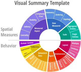
Visual summary diagrams are used to illustrate the content of a piece of literature according to our taxonomy, and idea adopted from Mason et al. [41]. Within the diagram, visual ele-ments (arranged colored shapes) represent categories, and the overall design of the visual summary illustrates the structure of the categories found for a field (see Section4.8for a discussion on the design choices underlying the final diagram). Categories present within the paper have the corresponding visual element highlighted, while those not present are made less visible (but still legible, to give context of what was not contained within a pa-per). Thus, a new visual summary diagram is created for each piece of literature reviewed (see Appendix A: Additional Visual Summaries for examples) which shows the subjects (categories) covered within the specific text. This allows for an at-a-glance evaluation of how individual papers approach the field. Figure2shows our resultant visual summary template for the entire field of spatial measures and behavior (i.e., the categories identified within existing literature).

4

Results and discussion

included, which includes topics we expected to find but that no current literature appears to address. We also build upon Mason et al.’s method by increasing the use of validation tasks, including using a naïve rater, to ensure that the categories were not arbitrary or id-iosyncratic to the authors. We will also discuss the visual design of the visual summary diagram itself. We walk through an example visual summary for O’Neill [49] to give a practical example of how categories are assigned. We then discuss our implementation of a web interface that allows users to create their own visual summaries and contribute to the corpus. Finally, two example use cases are discussed to illustrate how visual summaries can be used for research tasks.

Figure 2: The final visual summary template for spatial measures and human behavior research.

4.1

Category definitions

on the other hand refers to a specific, distinguishable part of a space. This part may be a specific (geographic) object, such as a piece of furniture within a room, a room within a building, a building on a campus, or a district of a city. It can also be generic, referring to location within a space that is not further explicitly specified.

In a case where a paper re-uses data from a previous study, that use is treated identically to if it were original as a practical matter. Research that analyzes data from previous studies or experiments and then also compares it with original data (data collected by the authors specifically for the research conducted in the paper) is classified by taking the pre-existing study or studies into consideration together with the new contribution. An example of this occurs in Turner and Penn [60], in which the authors correlate the results of an arti-ficial agent model to results of a previous study tracking the movement of human agents conducted by Hillier et al. [28]. In the classification, this would result in the paper being categorized as having both artificial and human agent (along with any other applicable category).

4.1.1 Spatial measures

Measured aspect Beginning at the left of the diagram (Figure2) and moving clockwise, the first superordinate category within the Spatial Measures domain is measured aspect, which represents what the spatial measure within an article means or intends to capture about a space or entity. The subcategories are centrality, saliency, visibility, and complex-ity/cost.

Centralityrefers to the importance of an entity based on its spatial relation with other entities. It can be established for structured (e.g., networks) and unstructured spaces. Cen-trality can be local (based on information of surrounding entities selected by some criteria) or global (based on information of all entities in a space). For example, Baran, Rodríguez, and Khattak [3] compared space syntax measures of local and global centrality to walking behavior in different neighborhoods.

Saliencyrefers to the distinctiveness or identifiability of an entity, relative to other enti-ties. Nothegger, Winter, and Raubal [46], for example, developed a model that uses various attributes, such as color and facade area, to create a single measure of saliency for buildings.

Visibilityrepresents measures that capture the degree of visibility between one or more entities to or from another entity or set of entities. This is what Benedikt [5] used in creating a series of isovist measures to quantify the nature of visible space around a single point, as well as proposing a series of methods to quantify visibility continuously across space.

Cost/complexityrepresents how comprehensible the internal structure of a space is (i.e., how easy it is to understand a space) or the mental or physical difficulty of traversing a space (i.e., how easy it is to navigate and/or move through a space to a desired destina-tion). Measures that attempt to measure cost/complexity are often derived from a space’s components. O’Neill [49], for example, was interested in the effect of average intersection complexity on wayfinding task performance in relatively small scale spaces (sections of a library). Richter [52] combined different aspects of a road intersection (such as number of branches and segment lengths) to define a measure for that intersection’s cognitive com-plexity.

environ-mental aspects, including visibility, to yield a landmark saliency measure. In that case, the paper is considered in the classification to include both saliency and visibility as the measured aspects.

How measured? How measuredis the second superordinate category, which captures the actual mathematical structure used to derive values, outside the context of what aspect is being measured. This category is important to classify basic information about methodolo-gies outside the intention of the measure.

The geometry category accounts for quantitative (numeric) measuring of geometric properties such as shape, size, angle, and metric distance. Examples include angular change [1,60], and metric distance [45].

Ordering refers to measures which assess linear/circular order of a finite number of entities, also without measuring metric properties of distance or angle. Richter and Klip-pel [53], for example, use circular ordering information of an intersection’s branches and the position of a landmark object within that order to determine that landmark’s location relative to a turn at the intersection (e.g., whether a landmark is located before or after the turn).

The categorytopologyrepresents measures of spatial relationships between entities in terms of connectedness or neighborhood without regard for geometric properties like met-ric distance, angle, size, or shape. For example, Hölscher, Brösamle, and Vrachliotis [29] identify areas of high centrality, using space syntax measures, which abstract a space into a graph. This graph abstraction allows for the purely topological relationships of the areas within a space to be quantified, such as how connected they are to other areas, without regard for geometric properties like metric distance.

Scale Scale, the last superordinate category within the spatial measures domain, indicates whether a measure operates on an entire space or part of it. Note this is not scale in the sense of map scale, and does not describe the size of the space.

The category ofaggregated entitiescaptures measures that summarize values from a mea-sure for individual entities into (usually) a single meamea-sure for a larger unit. That is, sum-marizing measures for individual intersections to a single measure for the whole route, or calculating an average measure for a larger area from values for individual locations within that area. An example of this is O’Neill’s [49] global ICD, which summarizes the complex-ity of a space based on aggregating the number of decisions available at all intersections within a space, resulting in a single (average) value for that space.

Single entities, on the other hand, comprises measures which provide values for indi-vidual entities of a space and, thus, reveal differences between them. For instance, Baran, Rodríguez, and Khattak [3] use an axial line map and integration to yield a centrality value for each axial line, which defined segments of a pedestrian path network.

4.1.2 Behavior

Human context Beginning from the left and moving counterclockwise,human context cap-tures studies which collect additional information on the characteristics of participating human agents, such as familiarity, expertise, sex, or individual differences. Nothegger, et al., [45], for example, had human agents with varying degrees of reported familiarity with the study area identify landmarks at street intersections within the study area. These were then compared to landmarks which were defined as salient by an algorithm constructed for that purpose.

Collection The superordinate category ofcollectioncaptures the two general ways behav-ioral data is gathered.

The first category isexperimental, which refers to data recorded by researchers in an original study described in their paper. In papers categorized as such, researchers manip-ulate variables, such as the environment participants operate in, or the kind of informa-tion presented to participants, or the kind of participants, to observe causal relainforma-tionships. O’Neill [49] once again provides an example of this, in performing an original wayfinding experiment that was conducted with human agents.

In contrast,non-experimentalcaptures papers whose methodology is outside the realm of experimental research. In those papers, data is collected without the controlled manipu-lation of variables, such as with a survey, an observational study, or census data. Koohsari et al. [33] is an example, utilizing mailed surveys that asked human agents to report how often they walked to nearby public open spaces (i.e., parks) and how much time they spent doing so.

Behavioral data The third superordinate category in this domain isbehavioral data, which stands for the type of data that captures the behavior of agents in some quantifiable way. It contains four categories.

The first isrecall; evaluations of how well a space and/or entities within that space are remembered by agents. This is measured post-hoc, that is, after some task execution. It may be measured on different levels of spatial knowledge, such as landmark, route, or survey. An example of research fitting into recall comes from Omer and Goldblatt [48], who had human agents mark the location of landmarks on an incomplete map of a space in which they had previously performed wayfinding tasks.

The second category ispreference, which accounts for research in which agents indicate a preference given a set of choices, as in Weisman [64]. That paper described a task in which human agents judge a series of highly abstracted floor plans in terms of their level of general preference for the plan.

The third category isuncontrolled, which represents when research tracks an agent’s de-cisions without a specific goal imposed upon the agents by the researchers. The researchers do not measure performance (of any kind), but simply observe behavior, such as how many agents pass by or enter a specific location, such as in Chang [12], who observed pedestrian movement by creating “gates” at particular points in a physical space and measured how many human agents passed through them. In addition, human agents passing through the gates were randomly selected and their movement tracked through the space.

ability to find a predetermined destination was measured in three ways: 1) time elapsed, 2) number of backtracks on route, and 3) number of wrong turns.

Agent The superordinate category Agent accounts for research using different beings whose behavior or actions are observed (and compared to particular spatial measures).

Naturalcaptures research which uses human agents, people used as test participants, as in O’Neill [49], which had students perform wayfinding tasks.

On the other hand,artificial, represents research which uses agents whose actions are intended to approximate human behavior, as in Turner and Penn [63], who used an agent-based model in which the agents used visibility information to make movement decisions.

Environment Environmentis the next superordinate category and represents the different ways environment/spaces are experienced in the study by agents.

First, research can usephysical spaces, an actual physical space as it exists in the real world, as in O’Neill [49], who had agents perform tasks in a university library building.

Second, there arevirtualenvironments, which are computer-generated spaces with or without the rules of physical reality, such as a digital three-dimensional model of a campus. One example of this is Meilinger, Franz, and Bülthoff [42], who had human agents experi-ence a three-dimensional simulation of a town through an immersive220◦semi-cylindrical screen.

The last environment category is external representation. This represents studies that utilize an (often static) representation of a space, such as a floorplan, map, or series of photographs, in addition to (or instead of) having agents interact in or move within a real or simulated environment. Asami et al. [1] had designated experts select local centers in Istanbul using a map of the city. O’Neill [49] had both “physical” and “external represen-tation” environments. Human agents first experienced the environment through the use of a series of photographs in order to familiarize them with the space before encountering it physically.

Layout The last superordinate category within behavior islayout, which captures the type of spatial structure or arrangement of the environment used within a paper.

The first isexisting, which refers to a spatial layout found in the real world that could be encountered in life, such as a street grid of a real place. For example, Hölscher, Brösamle, and Vrachliotis [29] had human agents perform tasks within a pre-existing building (a con-ference center), while Meilinger, Franz, and Bülthoff [42] had human agents experience a

virtualmodel of the town of Tübingen, Germany.

The second category issynthetic, which stands for when a paper uses a layout that is designed specifically to test behavioral responses to environmental aspects, such as a maze or idealized rectilinear street network. Dalton [15] did this by creating a virtual, idealized urban form consisting of streets of all the same length, but a variety of intersection types, which human agents then experienced through a computer simulation.

4.2

Considered categories

Over the course of affinity diagramming many categories were created, deleted, and re-vised. Importantly, there were categories we expected to find, and ways we anticipated to structure the taxonomy that did not hold up under a close reading of the corpus. Some absent categories seem to indicate there are under-researched areas that can be identified with this method. If they begin to materialize in the literature, the taxonomy and visual summary diagram can be updated accordingly (a possibility further discussed in Section5). One notable example of a conceptually sound category that was not present in the lit-erature was three-dimensional spatial measures. Three dimensional measures seem to be a neglected aspect of spatial measures research, especially in the face of the increasing com-monality of three-dimensional geospatial data, particularly for urban environments [34]. While many of the papers attempted to capture three-dimensional information, this gen-erally entailed abstracting the environment so that a two-dimensional measure could be used. An example of this can be seen in Hölscher, Brösamle, and Vrachliotis [29], who ana-lyzed multiple floors of a building together by creating “dummy” connections to simulate them all being on the same level.

Another example was dynamic layouts. Currently all encountered research seems to assume that effectively an environment is static, or at least does not meaningfully change during a task such as navigation. Conceptually, it is not difficult to imagine an environment where the navigable space changes quickly, such as a maze with moving walls. Obviously, this would be easier to implement experimentally in a virtual environment, but there are real-life situations where the environment is dynamic, such as a street network prone to accidents, or a burning building.

Some of the discarded categories had roots in common sense, but upon closer examina-tion were too difficult to define satisfactorily. We make the assumpexamina-tion that if we cannot effectively create a logically consistent definition, then a user will have an even harder time parsing or applying it. Several proto-categories cut for this reason fell under a su-perordinate category titledabstraction(orentity type). This would have referred to the base data type of the representation, or the type of abstraction from the real world. Lynch [39], for example, distinguishes paths, edges, districts, nodes, and landmarks. Golledge [22] provides geometric components of spatial knowledge as points, lines, areas, and surfaces. While common conceptually, actually distinguishing the different types within the litera-ture is nontrivial. Several common measures operate partly by transforming between such abstractions, such as axial line mapping in space syntax, which uses a linear representation to then define a network on which graph measures are calculated [27]. In a similar vein, isovist fields [4], account for various polygonal metrics for visibility at every point in a space.

We were cognizant of the difficulty in creating objective criteria for assigning categories given these complexities, and then informing users of these criteria. Accordingly, it was decided to instead focus on the intent of the measures and only provide high level in-formation in regards to methodology. This is represented in themeasured aspectandhow measuredsuperordinate categories, respectively. Another revision was to changeglobaland

scales. For example, when does one move from a neighborhood to a district, or from a city to region?

4.3

Validation of categories

In order to verify the applicability of the proposed categorization, we undertook three dif-ferent literature classification tasks for which inter-rater agreement was quantified via Co-hen’s Kappa [13]. Cohen’s Kappa accounts for agreement that could be expected by chance alone. Two rounds of classification were completed among three of the authors, with a third round using one author and one outside “naïve” rater only somewhat familiar with the research area (a cognitive neuroscientist).

Kappa

Statistic <0.00 0.00–0.20 0.21–0.40 0.41–0.60 0.61–0.80 0.81–1.00 Strength of

Agreement Poor Slight Fair Moderate Substantial

Almost Perfect

Table 1: Guidelines for interpreting Cohen’s Kappa values [25].

Author-only classifications directly informed revisions to the categories. Ten papers were independently classified in the first round, using a set of preliminary definitions cre-ated in the affinity diagramming method described in Section3.1. The authors’ results were compared pairwise, with the following Cohen’s Kappa values for each of the three pairs: 0.66,0.65, and0.60. These values fall between “Moderate” and “Substantial” according the guidelines for interpreting Cohen’s Kappa provided by Landis and Koch [35] (see Ta-ble1). This indicated the classification was not mature, and repeated disagreements, such as consistent differences for particular categories, were analyzed and discussed, and the classification revised. Some of the details of this discussion and its results are examined in Section4.2. Once the revision of the categories was complete, a second round using three papers was completed. This was considerably more successful, with two pairs recording identical Cohen’s Kappa of0.80(extreme high end of “substantial”) and one pair returning a result of0.94(“almost perfect”) [35]. After a discussion, which focused on understand-ing the remainunderstand-ing disagreements, and small follow-up revisions to definitions includunderstand-ing examples for each category, the naïve rater evaluation began.

Table 2: Results of the naïve rater task. Green shows agreement on assigning a paper to a category, blue shows agreement on not assigning a paper to a category, and orange shows a disagreement on whether or not to assign a paper to a category.

4.4

Example visual summary

Figure 3: An example visual summary created for O’Neill [49].

Beginning from the top left of the visual summary (Figure3), this paper has complex-ity/costas ameasured aspect, as the ICD measure O’Neill uses is intended to summarize the complexity of the environment. ICD does this by simple topology, summarizing the degree of nodes (intersections; termedchoice points) in the floorplan of the environments. Thus, the

topologyandhow measuredcategories are highlighted. Since the measure aggregates the val-ues of all the choice points in an environment rather than singling out any individual value,

scaleandaggregated entitiesare highlighted. Forlayout,multipleis flagged because three dif-ferent environments within the library (with difdif-ferent complexity) were evaluated.Existing

is flagged because these environments already existed and were not designed for the task by the researcher. Forenvironment, the library settings were physical spaces (as opposed to virtual), thusphysicalis highlighted. External representationis also flagged because O’Neill used a series of photographs to give a “guided tour” of the environment to participants as a pre-training task before the wayfinding component of the experiment.

The participants were graduate and undergraduate students, sonaturalis marked under

envi-ronment they navigated, and evaluated that map for completeness and accuracy. O’Neill explicitly conducted an experiment (rather than a survey or other method), socollection

andexperimentalare flagged. Since O’Neill did not compare any aspect of the participants (such as age, gender, or experience) other than the results of their experimental task,human contextremains un-flagged.

4.5

Web-based classification and analysis tool

In order to simultaneously bring our results to a wider audience of scholars and to build our knowledge base, we are in the final stages of implementing a web interface for both exploring and creating visual summaries.1_{Once a user is registered, they can create visual}

summaries for new papers and add their bibliographic information via BibTex [18], which is then added to the corpus database. The intent is that this approach will function as a form of crowdsourcing, increasing the size (and therefore utility) of our corpus, and opening up opportunities for future analysis.

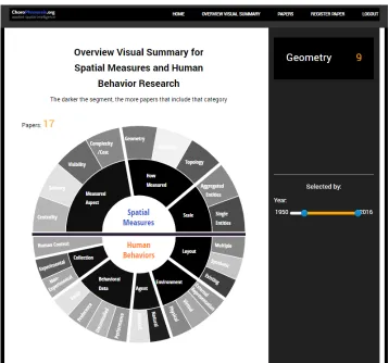
Users can browse the existing database of visual summaries, and select papers by cate-gory, so that only papers with the selected categories are displayed. An example use-case of this feature is given in Section4.6. In addition to manual visual comparison, the website also has an interactive overview visual summary. Intended to give users a sense of larger trends, this displays how often categories are present within the entire corpus database, or a selection of that database. A screenshot of the current status is shown in Figure4. Darker segments indicate more popular categories.

Currently, users can select to show only papers within a date range (by year of publica-tion), which can give an indication of trends by simply changing the selected range. More selection features are planned, such as being able to select by author name.

4.6

Example use cases

One major strength of using a diagram to represent categories is that it makes comparing literature straightforward. An example use case would be a researcher who is familiar with a specific body of research, but looking to explore whether a specific idea has been pursued outside that body. Using our web interface, they could select their topics of interest. For example, they could be interested in the visibility of landmarks in virtual reality, and select the appropriate subordinate categories (visibility and virtual). In the results, they could look for unfamiliar names or unusual combinations of categories (such as the use of non-experimental data collection).

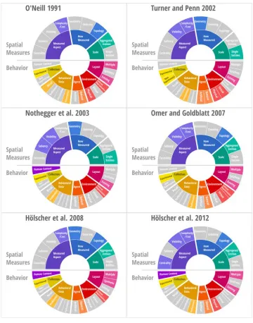
Let us now take the perspective of another user, a first-semester graduate student who is interested in work that examines navigational difficulty based on environment com-plexity for the purposes of planning an experiment to base their thesis around. Using our website, they query for literature that has complexity/cost measures andexperimental

data collection. The visual summaries in Figure 5 are shown: O’Neill [49], Turner and Penn [63], Dalton [14], Omer and Goldblatt [48], and two papers by Hölscher with different co-authors [29,30].

Several patterns can be noticed immediately within the selected categorizations. First,

complexity/costis often investigated jointly withvisibility, but never withcentrality. Ordering

1_{For the current state of implementation, seehttp:chorophronesis-magicat.rhcloud.com/visualsummary/}

Figure 4: Screenshot of web interface. The overview visual summary for all papers, as shown in our web interface (in progress). The darker the segment, the more papers that contain that category. Users can mouse over segments to get an exact count of papers that include it (displayed top right). Users can also use an interactive timeline to restrict the display by publication year. Other features are planned, such as query by author name.

never appears, perhaps indicating that using it as an approach could be novel in this con-text. Most research usesaggregated entities, but not all. All collection isexperimental(since this was one of the query terms), but one paper supplements this with non-experimental

data collection. The actual type of behavioral information collected varies considerably, perhaps indicating to our graduate student that they need to consider the type of data they would like to collect to refine their search (such as focusing onperformance).Naturalagents (people) might be expected, but perhaps the only paper to useartificialagents (Turner and Penn’s) might provide some insight as to how they can be employed. Similar to behav-ioral data used, the type of environment varies, indicating another area that requires some thought for further specification. Half of the papers examine bothmultiple and existing

Figure 5: An illustration of how multiple visual summaries can be used to compare papers quickly. All papers share the categories of Complexity/Cost and Experimental (collection).

theme). However, the lack of papers that have attempted to use or compareexistingand

While this example may be a somewhat idealized scenario, we believe it nicely illus-trates the possibilities of our visual summary output for identifying themes and potential avenues for future research.

4.7

Why not automated text analysis?

The modified affinity diagramming method used by Mason et al., and modified here, is used in lieu of automated text analysis methods. This is primarily because we feel they would not function well for our particular purpose: creating a robust taxonomy for a highly interdisciplinary domain whose core literature set is not intractably large. Automated text analysis methods still require humans to provide domain knowledge [21,23], whether they are used to identify topics within literature or assign topics (categories) to literature. In un-supervised classification a person is still needed to make sense of the output of discovered patterns, such as nominal topics [43]. Our analysis, i.e., the creation of categories, is most closely analogous totopic modeling, the various approaches aimed at automatically extract-ing “topics” from text corpora. For overviews on topic modelextract-ing, see, for example, Mohr and Bogdanov [43] and Brett [10].

Similarly, automated assignment of categories of literature (a classification problem) re-quires a person to define the categories to apply, and often to classify papers in order to create a training set for the model [23]. Given that we are faced with a corpus that is both comparatively small and rather heterogeneous, the effort needed to fine-tune automated methods or training sets for them to produce sensible categorizations seems unnecessary and wasted, particularly given that they would still be unlikely to capture all intricacies and seeming contradictions in term use, for example. Theoretically the affinity diagram-ming method does not even require the use of a computer, which is advantageous where resources are limited or there is a lack of technical expertise. Still, the use of automated methods for visual summaries may prove to be especially useful in some scenarios, an idea we discuss in Section5.

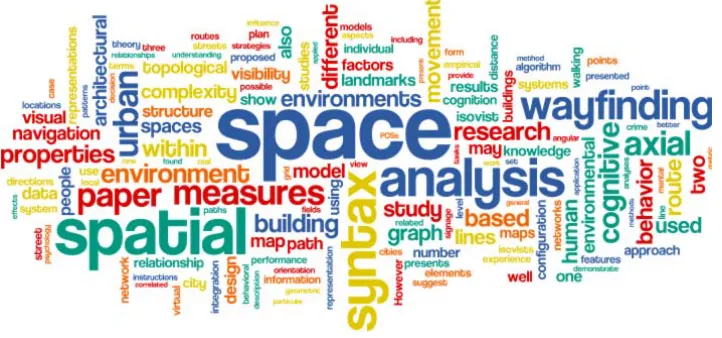
The advantages of the combination of affinity diagramming and visual summary can further be seen when compared with a word cloud, a basic form of text analysis. A word cloud displays common words from a text source, with the larger font used corresponding to more common words (barring common words in English syntax). An example word cloud created usingwww.wordle.net[19] is shown in Figure6. The text used was the ab-stracts from a selection of our corpus (the same selection is used in Appendix A: Additional Visual Summaries).

A word cloud is a simplistic form of text analysis, but it clearly illustrates a funda-mental challenge: the difference between words (as a group of characters) and their actual meaning. For example, “graph” and “network” can be synonymous, or have completely different meanings, depending on the context (i.e., a statistical graph). This specific exam-ple is also discussed by Borrett et al. [3], who in the context of analyzing network ecology literature had to adjust for multiple keywords and spurious phrases that included related terms but were not directly of interest, such as “transportation network.”

manu-Figure 6: A word cloud made using abstracts of literature within our corpus.

ally, especially in an interdisciplinary context, is that it inherently allows content and ideas to be disconnected from the specific language used to describe them. This aspect cannot currently be achieved with automated text analysis approaches of any kind.

4.8

Visual summary design

The design of the visual summary can be seen in Figure2. According to Mackinlay [40], the two most effective visual variables [6] for “perceptual tasks” using nominal data are posi-tion and color hue. We focus on these two elements to represent the categorical meaning of the elements in the diagram, while attempting to control for other visual variables, such as size, and maintaining an aesthetic balance.

First, the diagram is split into two halves: the top half containing spatial measures categories and the bottom half containing human behavior categories. The summary is hierarchical from the inside out, so that the outside categories (represented with “slices”) are subordinate to the inside categories. While the number of categories contained within each half is different, we felt it was important to keep the halves the same overall size to avoid the user assuming differing importance. Related category segments are grouped to-gether, but not ordered. The inner ring of segments contains the superordinate categories, while the outer ring contains subordinate categories. The sizes of the segments are deter-mined by the subordinate categories, so that all subordinate categories are the same size within each half. Superordinate categories are then sized to match the number of subordi-nate categories they contain. This leads to some superordisubordi-nate categories appearing bigger than others. This may imply differing importance to some, but on the other hand ensures that subordinate categories—which are more salient—keep the same size, and text in the diagram remains readable while the overall diagram still has a reasonable size.

cate-gory groups, with all the subordinate categories having the same color (to avoid indicating importance), and the superordinate category segment having a slightly darker tone. The circular shape was chosen to allow for segments to be added and removed in case of future revisions, without a need for a complete redesign. For example, ifdynamicenvironments as discussed in Section4.2were to be covered in future literature, they may be added to the “Environment” slice.

The visualization was refined and designed as the categories were refined. The empha-sis of the design is on clarity of information. Having a working visualization also helped to find the right level of granularity of representation for the intended purpose. Too general and the diagram fails to provide useful information; too detailed and users will have dif-ficulty finding what they are looking for. Two levels of hierarchy were selected over more detailed alternatives, since we believe this is a reasonable balance between visual search difficulty and level of detail.

5

Future work

The inter-rater agreement tasks speak to the validity of our taxonomy, and we believe the visual summary provides a valuable way to access and understand that categorization. However, there are opportunities for future research, both in terms of extending and ap-plying our existing visual summary and taxonomy, and improving the method.

As discussed in Section4.5, we are finalizing the implementation of a web interface for our visual summary of spatial measures and human behavior research. The site will allow scholars to view existing visual summaries, get an overview of frequency of categories in the database, and create their own visual summary for a given paper, which automatically adds that paper to the database. While currently the analytical features are still limited, we are planning to implement more advanced tools. There are many classic bibliometric analyses that would be interesting to combine with the categorical information of our tax-onomy. For instance, which journals or authors are associated with which categories, and how those associations change over time.

The web interface offers more opportunities for further evaluations of the taxonomy and the visual summary. For example, crowdsourcing-style evaluations of the taxonomy could be performed by asking multiple users to classify the same papers and then compar-ing their mutual agreement across papers and categories. In theory, an automated system for creating visual summaries makes creating different representations of the same data relatively easy, making an evaluation of different visualization methods possible.

updated automatically within the web interface. In the unlikely event that new categories are found which require a complete review of the existing corpus, a manual review would be necessary, which would be time consuming but not impractical.

While we have discussed the advantages of using the modified affinity diagramming method over automated text mining, we believe there might be potential in exploring ma-chine learning methods to support the categorization process. For example, cluster analysis could be used to help find previously unrecognized subfields of research, or jump start the categorization process, especially for broader or more complex fields. Despite the potential of extending the method, we believe the current iteration provides a helpful, easy to com-prehend way to both create an understanding of a field of literature (through the creation of categories) and communicate that understanding in an effective way that enhances readers’ understanding of single papers and entire fields.

Acknowledgments

We would like to thank Qingyu Ma for his invaluable work on the web interface. The US authors would like to acknowledge funding through the National Science Foundation grant #1526520.

References

[1] ASAMI, Y., KUBAT, A. S., KITAGAWA, K., ANDIIDA, S.-I. Introducing the third di-mension on space syntax: Application on the historical Istanbul. InProc. 6th Interna-tional Space Syntax Symposium(Istanbul, Turkey, 2007), A. S. Kubat, Ed., ITU Faculty of Architecture, pp. 48.1–48.18.

[2] BAFNA, S. Space syntax: A brief introduction to its logic and analytical techniques.

Environment and Behavior 35, 1 (2003), 17–29.doi:10.1177/0013916502238863.

[3] BARAN, P. K., RODRÍGUEZ, D. A.,ANDKHATTAK, A. J. Space syntax and walking in a new urbanist and suburban neighbourhoods. Journal of Urban Design 13, 1 (2008), 5–28. doi:10.1080/13574800701803498.

[4] BATTY, M. Exploring isovist fields: Space and shape in architectural and urban morphology. Environment and Planning B: Planning and Design 28, 1 (2001), 123–150. doi:10.1068/b2725.

[5] BENEDIKT, M. L. To take hold of space: Isovists and isovist fields. Environment and Planning B: Planning and Design 6, 1 (1979), 47–65.doi:10.1068/b060047.

[6] BERTIN, J.Semiology of Graphics: Diagrams, Networks, Maps, 1st ed. ed. ESRI Press and Distributed by Ingram Publisher Services, Redlands, Calif., 2010.

[8] BORRETT, S. R., MOODY, J.,ANDEDELMANN, A. The rise of network ecology: Maps of the topic diversity and scientific collaboration. Ecological Modelling 293(2014), 111– 127.doi:10.1016/j.ecolmodel.2014.02.019.

[9] BOYACK, K. W., KLAVANS, R.,ANDBÖRNER, K. Mapping the backbone of science. Scientometrics 64, 3 (2005), 351–374.doi:10.1007/s11192-005-0255-6.

[10] BRETT, M. R. Topic modeling: A basic introduction. Journal of digital humanities 2, 1 (2012), 12.

[11] CARLSON, L. A., HÖLSCHER, C., SHIPLEY, T. F., AND DALTON, R. C. Getting lost in buildings. Current Directions in Psychological Science 19, 5 (2010), 284–289. doi:10.1177/0963721410383243.

[12] CHANG, D. Spatial choice and preference in multilevel movement networks. Environ-ment and Behavior 34, 5 (2002), 582–615.doi:10.1177/0013916502034005002.

[13] COHEN, J. A coefficient of agreement for nominal scales.Educational and Psychological Measurement 20, 1 (1960), 37–46.doi:10.1177/001316446002000104.

[14] DALTON, R. C. The secret is to follow your nose: Route path selection and angularity.

Environment & Behavior 35, 1 (2003), 107–131.doi:10.1177/0013916502238867.

[15] DALTON, R. C., HÖLSCHER, C.,ANDTURNER, A. Understanding space: The nascent synthesis of cognition and the syntax of spatial morphologies. Environment and Plan-ning B: PlanPlan-ning and Design 39, 1 (2012), 7–11.doi:10.1068/b3901ge.

[16] DARA-ABRAMS, D. Cognitive surveying: A framework for mobile data collection,

analysis, and visualization of spatial knowledge and navigation practices. InSpatial cognition VI, C. Freksa, Ed., vol. 5248 ofLecture notes in computer science, 0302-9743. Springer, Berlin, 2008, pp. 138–153. 10.1007/978-3-540-87601-4doi:\textunderscore12.

[17] EVANS, G. W. Environmental cognition. Psychological Bulletin 88, 2 (1980), 259–287. doi:10.1037/0033-2909.88.2.259.

[18] FEDER, A. Bibtex.http:www.bibtex.org/, 2016. Last accessed 10 December 2016.

[19] FEINBERG, J. Wordle - create. http:www.wordle.net/create, 2016. Last acccessed May 4 2016.

[20] FRANZ, G.,ANDWIENER, J. M. From space syntax to space semantics: A behaviorally and perceptually oriented methodology for the efficient description of the geometry and topology of environments. Environment and Planning B: Planning and Design 35, 4 (2008), 574–592.doi:10.1068/b33050.

[21] FUCHS, G., STANGE, H., SAMIEI, A., ANDRIENKO, G.,ANDANDRIENKO, N. A semi-supervised method for topic extraction from micro postings.it - Information Technology 57, 1 (2015).doi:10.1515/itit-2014-1078.

[23] GRIMMER, J.,ANDSTEWART, B. M. Text as data: The promise and pitfalls of automatic content analysis methods for political texts. Political Analysis 21, 3 (2013), 267–297. doi:10.1093/pan/mps028.

[24] HALLOWELL, G. D., ANDBARAN, P. K. Suburban change: A time series approach to measuring form and spatial configuration. The Journal of Space Syntax 4, 1 (2013), 74–91.

[25] HARDY, A. C. Landscape and human perception.Methods of Landscape Analysis Octo-ber(1967), 3–8.

[26] HILLIER, B. Space is the Machine: A configurational theory of architecture. Cambridge University Press, Cambridge, 1996.

[27] HILLIER, B.,ANDHANSON, J. The Social Logic of Space. Cambridge University Press,

Cambridge, 1984.

[28] HILLIER, B., MAJOR, M. D., DESYLLAS, J., KARIMI, K., CAMPOS, B.,ANDSTONOR, T. Tate Gallery, Millbank: A study of the existing layout and new masterplan proposal. Tech. rep., Bartlett School of Graduate Studies, University College London, London, UK, 1996.

[29] HÖLSCHER, C., BRÖSAMLE, M., AND VRACHLIOTIS, G. Challenges in multilevel

wayfinding: A case study with the space syntax technique. Environment and Planning B: Planning and Design 39, 1 (2012), 63–82.doi:10.1068/b34050t.

[30] HÖLSCHER, C.,ANDDALTON, R. C. Comprehension of layout complexity: Effects of

architectural expertise and mode of presentation. InDesign Computing and Cognition ’08, J. S. Gero and A. K. Goel, Eds. Springer, Dordrecht and London, 2008, pp. 159–178. 10.1007/978-1-4020-8728-8doi:\textunderscore9.

[31] JIANG, B. Ranking spaces for predicting human movement in an urban

environ-ment. International Journal of Geographical Information Science 23, 7 (2009), 823–837. doi:10.1080/13658810802022822.

[32] KOHONEN, T. Essentials of the self-organizing map. Neural networks 37(2013), 52–65.

doi:10.1016/j.neunet.2012.09.018.

[33] KOOHSARI, M. J., KACZYNSKI, A. T., GILES-CORTI, B., AND KARAKIEWICZ, J. A.

Effects of access to public open spaces on walking: Is proximity enough? Landscape and Urban Planning 117(2013), 92–99.doi:10.1016/j.landurbplan.2013.04.020.

[34] LAFARGE, F.,ANDMALLET, C. Creating large-scale city models from 3d-point clouds: A robust approach with hybrid representation.International Journal of Computer Vision 99, 1 (2012), 69–85.doi:10.1007/s11263-012-0517-8.

[35] LANDIS, J. R.,ANDKOCH, G. G. The measurement of observer agreement for cate-gorical data.Biometrics 33, 1 (1977), 159.doi:10.2307/2529310.

[37] LI, R.,ANDKLIPPEL, A. Wayfinding behaviors in complex buildings: The impact of environmental legibility and familiarity. Environment and Behavior 48, 3 (2016), 482– 510.doi:10.1177/0013916514550243.

[38] LU, Y., AND ZIMRING, C. Can intensive care staff see their patients? An im-proved visibility analysis methodology.Environment and Behavior 44, 6 (2012), 861–876. doi:10.1177/0013916511405314.

[39] LYNCH, K.The Image of the City. MIT Press, Cambridge, MA, 1960 (1975).

[40] MACKINLAY, J. Automating the design of graphical presentations of relational infor-mation. ACM Transactions on Graphics 5, 2 (1986), 110–141.doi:10.1145/22949.22950.

[41] MASON, J. S., RETCHLESS, D.,ANDKLIPPEL, A. Domains of uncertainty visualiza-tion research: A visual summary approach. Cartography and Geographic Information Science(2016), 1–14. doi:10.1080/15230406.2016.1154804.

[42] MEILINGER, T., FRANZ, G.,AND BÜLTHOFF, H. H. From isovists via mental

repre-sentations to behaviour: First steps toward closing the causal chain. Environment and Planning B: Planning and Design 39, 1 (2012), 48–62.doi:10.1068/b34048t.

[43] MOHR, J. W., ANDBOGDANOV, P. Introduction—topic models: What they are and why they matter.Poetics 41, 6 (2013), 545–569.doi:10.1016/j.poetic.2013.10.001.

[44] MONTELLO, D. R. The contribution of space syntax to a comprehensive theory of environmental psychology. InProc. 6th International Space Syntax Symposium(Istanbul, Turkey, 2007), A. S. Kubat, Ed., ITU Faculty of Architecture, pp. iv.1–iv.12.

[45] NAGAR, A., ANDTAWFIK, H. A multi-criteria based approach to prototyping urban road networks.Issues in Informing Science and Information Technology Education 4(2007), 749.

[46] NOTHEGGER, C., WINTER, S., AND RAUBAL, M. Selection of salient fea-tures for route directions. Spatial Cognition and Computation 4, 2 (2004), 113–136. 10.1207/s15427633scc0402doi:\textunderscore1.

[47] NUBANI, L.,ANDWINEMAN, J. The role of space syntax in identifying the relation-ship between space and crime. InProc. International Space Syntax Symposium (Amster-dam, Netherlands, 2005), A. van Nes, Ed., pp. 413–422.

[48] OMER, I., AND GOLDBLATT, R. The implications of inter-visibility between land-marks on wayfinding performance: An investigation using a virtual urban en-vironment. Computers, Environment and Urban Systems 31, 5 (2007), 520–534. doi:10.1016/j.compenvurbsys.2007.08.004.

[49] O’NEILL, M. J. Evaluation of a conceptual model of architectural legibility. Environ-ment and Behavior 23, 3 (1991), 259–284.doi:10.1177/0013916591233001.

[51] PEPONIS, J., ZIMRING, C., AND CHOI, Y. K. Finding the building in wayfinding.

Environment and Behavior 22, 5 (1990), 555–590.doi:10.1177/0013916590225001.

[52] RICHTER, K.-F.,ANDDUCKHAM, M. Simplest instructions: Finding easy-to-describe routes for navigation. In Geographic Information Science, T. J. Cova, Ed., vol. 5266 of Lecture notes in computer science, 0302-9743. Springer, Berlin, 2008, pp. 274–289. 10.1007/978-3-540-87473-7doi:\textunderscore18.

[53] RICHTER, K.-F., AND KLIPPEL, A. Before or after: Prepositions in spatially con-strained systems. InSpatial cognition V, T. Barkowsky, Ed., vol. 4387 ofLecture notes in computer science. Lecture notes in artificial intelligence, 0302-9743. Springer, Berlin, 2007, pp. 453–469. 10.1007/978-3-540-75666-8doi:\textunderscore26.

[54] SKEELS, M., LEE, B., SMITH, G., AND ROBERTSON, G. G. Revealing uncer-tainty for information visualization. Information Visualization 9, 1 (2009), 70–81. doi:10.1057/ivs.2009.1.

[55] SKUPIN, A., AND AGARWAL, P. Introduction: What is a self-organizing map? In

Self-organising maps, P. Agarwal and A. Skupin, Eds. Wiley, Chichester, England and Hoboken, NJ, 2008, pp. 1–20. doi:10.1002/9780470021699.ch1.

[56] SKUPIN, A., BIBERSTINE, J. R.,ANDBORNER, K. Visualizing the topical structure of the medical sciences: a self-organizing map approach. PloS one 8, 3 (2013), e58779. doi:10.1371/journal.pone.0058779.

[57] TANDY, C. R. The isovist method of landscape survey. Methods of Landscape Analysis

(1967), 9–10.

[58] THOMAS, J. J.,ANDCOOK, K. A. A visual analytics agenda. IEEE Computer Graphics and Applications 26, 1 (2006), 10–13.doi:10.1109/MCG.2006.5.

[59] TUFTE, E. R. The Visual Display of Quantitative Information, 2nd ed. ed. Graphics Press,

Cheshire, Conn, 2001.

[60] TURNER, A. Angular analysis. InProc. 3rd International Symposium on Space Syntax

(Atlanta, Georgia, 2001), Georgia Institute of Technology, pp. 30.1–30.11.

[61] TURNER, A. From axial to road-centre lines: A new representation for space syntax and a new model of route choice for transport network analysis. Environment and Planning B: Planning and Design 34, 3 (2007), 539–555.doi:10.1068/b32067.

[62] TURNER, A., DOXA, M., O’SULLIVAN, D., AND PENN, A. From isovists to visibil-ity graphs: A methodology for the analysis of architectural space. Environment and Planning B: Planning and Design 28, 1 (2001), 103–121.doi:10.1068/b2684.

[63] TURNER, A.,ANDPENN, A. Encoding natural movement as an agent-based system: An investigation into human pedestrian behaviour in the built environment. Environ-ment and Planning B: Planning and Design 29, 4 (2002), 473–490.doi:10.1068/b12850.

[65] WIENER, J. M., FRANZ, G., ROSSMANITH, N., REICHELT, A., MALLOT, H. A., AND

BÜLTHOFF, H. H. Isovist analysis captures properties of space relevant for locomotion and experience.Perception 36, 7 (2007), 1066–1083.doi:10.1068/p5587.

[66] WOLBERS, T.,ANDHEGARTY, M. What determines our navigational abilities? Trends in Cognitive Sciences 14, 3 (2010), 138–146.doi:10.1016/j.tics.2010.01.001.

Appendix B: Category Definitions

Essential idea:This classification’s central purpose is to help understand the state of the re-search literature regarding how quantifiable aspects of space influence human behavior in space. Accordingly, the classification is split into two major subsections: Spatial Measures and Behavior.

How to apply the classification scheme

• General advice:Be inclusive! Anything that you believe fits the study at hand should be marked in the classification. In particular, the following guidelines apply.

• Measures within measures:If authors measure some aspect by combining individual measures that cover other aspects, mark all these aspects in the classification (rather than just the ultimate result).

Example: Nothegger, Winter, and Raubal (2004) utilize several environmental as-pects, including visibility, to yield a landmark saliency measure. In that case, the paper is considered in this classification to include both saliency and visibility as the measured aspects.

• Pre-existing data:Research that analyzes data from previous studies or experiments and then also compares it with original data (data collected by the authors specif-ically for this research) is classified by taking the pre-existing study or studies into consideration together with the new contribution. That is, in the classification mark everything that applies either to the original data or the data from previous studies.

hu-man agents conducted by Hillier et al. (1996). In the classification, this would result in both artificial and human agent being marked, among others.

The classification scheme

In the explanations of the classification scheme’s elements we will use the terms “space” and “entity” to refer to elements of the (geographic) area research has been conducted in. The terms are used according to the following definitions:

• Space: “Space” refers to an area as a whole. This may be on different scales (e.g., a room, a building, a campus, a city. . . ), but it will usually be the encompassing area. “Space” may leave the internal structure of that area undefined.

• Entity:“Entity” refers to a specific, distinguishable part of a “space.” This part may be a specific (geographic) object, such as a piece of furniture within a room, a room within a building, a building on a campus, or a district of a city. It can also be generic, referring to a not further specified location within a space.

Elements of the classification scheme

Spatial Measures

Measured aspect The desired attribute of a space or entity, which measures are attempting to quantify.

• Centrality- Importance of an entity based on its spatial relation with other entities. It can be established for structured (e.g., networks) and unstructured spaces. Centrality can be local (based on information of surrounding entities selected by some criteria) or global (based on information of all entities in a space).

Example:Baran, Rodríguez, and Khattak (2008) compared space syntax measures of local and global centrality to walking behavior in different neighborhoods.

Asami et al. (2003) sought to identify the most central locations within historic Is-tanbul. They compared centers found using the space syntax measure of integration (which derive values for centrality based on the topology of the street network) to centers identified by experts using a map, by the number of taxi bays in an area, and by the average number of stories of buildings in an area.

• Saliency- The distinctiveness or identifiability of an entity, relative to other entities. Example: Nothegger, Winter, and Raubal (2004) developed a model that uses at-tributes, such as color and facade area, to create a single measure of saliency for buildings.

• Visibility- The degree of visibility between one or more entities to or from another entity or set of entities.

• Cost/Complexity- How comprehensible the internal structure of a space is (i.e., how easy it is to understand a space) or the mental or physical difficulty of traversing a space (i.e., how easy it is to navigate and/or move through a space to a desired destination). This is often derived from a space’s components.

Example:O’Neill (1991) was interested in the effect of average intersection complex-ity on wayfinding task performance in relatively small scale spaces (sections of a li-brary).

Richter (2009) combined different aspects of a road intersection (such as number of branches and segment lengths) to define a measure for that intersection’s cognitive complexity.

How measured? The actual mathematical structure used to derive values, outside the context of what aspect is being measured.

• Topology- Measures of spatial relationships between entities in terms of connected-ness or neighborhood without regard for geometric properties like metric distance, angle, size or shape.

Example:Hölscher, Brösamle, and Vrachliotis (2012) identify areas of high centrality, using space syntax measures, which abstract a space into a graph. This graph ab-straction allows for the purely topological relationships of the areas within a space to be quantified, such as how connected they are to other areas, without regard for geometric properties like metric distance.

• Ordering- Linear/circular order of a finite number of entities, without metric prop-erties of distance or angle.

Example: Richter (2007) uses circular ordering information of an intersection’s branches and the position of a landmark object within that order to determine that landmark’s location relative to a turn at the intersection (e.g., whether a landmark is located before or after the turn).

• Geometry- Quantitative (numeric) measuring of geometric properties such as shape, size, angle, and metric distance.

Example: Examples include angular change (Turner 2001, Asami et al. 2003), and metric distance (Nagar and Tawfik 2007).

Scale This refers to the scale a measure operates on, i.e., whether it operates locally or globally. Scaledoes notdescribe the size (or resolution) of the space.

• Aggregated Entities- Measures that summarize values measured for individual en-tities into (usually) a single measure for a larger unit (e.g., summarizing measures for individual intersections to a single measure for the whole route; calculating an average measure for a larger area from values for individual locations within that area).

• Single Entity- Measures which provide values for indi