Green's Function Theory for Ising Model in Transverse field for Arbitrary Spin

(1)

Green’s Function Theory for Ising Model in Transverse field

for Arbitrary Spin

Angel T. Apostolov*

1

_{, Iliana N. Apostolova}

2

*1_{University of Architecture, Civil Engineering and Geodesy, Faculty of Hydrotechnics, Hr. Smirnenski Blvd. 1, 1046 Sofia, Bulgaria} 2

University of Forestry, Faculty of Forest Industry, Kl. Ohridsky Blvd. 10, 1756 Sofia, Bulgaria

ABSTRACT

We have studied the transverse Ising system in terms of pseudo-spin variables S with arbitrary pseudo-spin using Green’s function technique and method proposed by Tserkovnikov. The phase diagrams, the longitudinal and the transverse polarizations are obtained. Numerical results are performed and analyzed for the particular cases S=3/2 and S = 2.

Keywords: Transverse Ising Model, Arbitrary Pseudo-Spin, Green’s function

I. INTRODUCTION

The Transverse Ising model (TIM) has been one of the most actively studied systems in statistical mechanics and has been used as an elementary model for a variety phenomenon. The TIM proposed by Blinc and de-Genne has been already investigated by the use of various techniques and approximations [1]. It has been applied to a wide variety of physical systems including order-disorder and displacive type ferroelectrics, induced moment ferromagnets and cooperative Jahn-Teller systems [2-4]. In the most of these applications, the operators are in the pseudo-spins presentation which describes the state of two-level systems, and the transverse field describes transitions between these levels. On the other hand, TIM for spin S higher than

S >1/2 has also received some attention. As far as we know, only a few works have made contact with the quantum spin-S TIM using high-temperature series, discretized path-integral representations or effective field theories [5-9]. Double-time Green's functions (GF) are used within a mean-field treatment for all spins of the two-sublattice TIM [10].

Over the last decade, Transverse Ising model for pseudo-spin S = 1/2 in combination with a modified Heisenberg model used to describe the mechanisms of magneto-electric coupling in the so-called multiferroics. They are materials which show spontaneous magnetic

and electric ordering in the same phase[11]. In many papers the electric properties in multiferroic EuTiO3 [12],

type-I multiferroics [13, 14], BiFeO3 [15], hexagonal

h-RMnO3 compounds [16], RMn2O5 [17] and composite

multiferroic thin films [18] are studied using the transverse Ising model with S = 1/2. This could be correct for example in the case of h-RMnO3 and RMn2O5.

The h-RMnO3 is a typical improper ferroelectric. The

polarization is produced by the uncompensated displacement of R ions along the c direction, where one-third of R ions shift upwards and two-thirds of R ions shift downwards, indicating that RMnO3 has two

opposite polarized states [19]. In the multiferroic state of

RMn2O5 with non-collinear Mn spin order and helical or

cycloidal geometry, the actual symmetry group is Pb21m, which allows for a macroscopic electric polarization along the b axis [17, 20]. But this is not the case in BiFeO3 (BFO). The structure of BFO which is a

lone pair multiferroic is characterized by two distorted perovskite blocks connected along their body diagonal denoted as pseudo-cubic [1,1,1] to build the rhombohedral unit cell [21, 22]. BFO exhibits both ferroelectricity and ferromagnetism, i.e. multiferroic with TC= 1100 K and TN= 643 K. The ferroelectric state

is realized by a large displacement of the Bi ions relative to the FeO6 octahedra, leading to the formation of eight

(2)

correspond to four structural variants (the polarization is along the four cubic diagonals) [22- 24]. This means that for the electric subsystem is more appropriate to describe using TIM with pseudo-spin S = 7/2.

The aim of the present paper is to create the self-consistent theory of TIM with arbitrary spin (S > 1/2) using retarded Green’s functions and method proposed by Tserkovnikov [25].

II. METHODS AND MATERIAL

The Ising model with transverse field Ω and correlated tunneling is defined by:

∑ ∑ ∑ (1) Here Ω is the transverse field (the tunneling frequency),

are the components of the pseudo-spins, Jijis the

exchange pseudo-spin interaction and Kij is the constant

of correlated tunneling. This Hamiltonian describes a phase transition different form pure Ising case. In all intervals of the tempetarure esixt an order . At high temperatures the Sz components are disordered and at temperatures below TC an ordered phase is

appeared with . The role of transverse field

Ω is to prevent this order. When Ω increases the transiton temperature decreases and at a given critical value ΩC transition temperature becomes zero. The last

term in equation (1) specifies the influence of the tunnel motion of a given particle on the tunnel motions of neighboring particles.

In order to observe the correlation functions, and the order’s parameters we use the retarded commutator Green’s function which is defined as [26]:

̂( ) ̂( ) ( )

[ ̂( ) ̂( )]

(2) We define the following GFs and the averages values of following commutators:

( )

0 ( ) 1

( )

0 ( ) 1 (3)

( )

0 ( ) 1

After time Fourier transformation the equation of motions and labor-intensive calculations for the GFs we get:

( )

( ) ( )

( )

( ) ( )

( )

(4) where ∑ , ∑

∑ and ∑

After solving these equations the ordered parameters and the pseudo-spin energy can be determined from the GF via the spectral theorem. A solution is possible by establishing a closed system of equations by decoupling the higher-order GF on the right side. For the exchange interactions, we use a generalized Tyablikov (or RPA) decoupling.

First, we will calculate and from the equation of motions:

[ ] [ ] .

The calculations show:

( ) (5)

then:

( ) ( )

(3)

(6)

Similarly:

( ) ( )

. ( ) ( ) / (7)

We define the following equations of motions: [ ] [ ]

[ ] . We get:

.

/ ( ) (8)

For ( ) using eq. 7 and eq. 8 we obtain:

( ) .

/ ( ) (9)

For the averages values: 0 ( ) 1

and

0 ( ) 1 we get:

0 ( ) 1 ,( ) ( ) -

,( ) ( ) -

If we take into account eq. 8 we have:

[ ( ) ] .

/ [( ) ( ) ]

( ) . (10)

Similarly:

[ ( ) ] ( ) ( )

If we take into account eq. 5 we get:

[ ( ) ]

( )

(11)

From eq. 3, eq. 10 and eq. 11 we have:

(

( )

( ) ( )

) (

)

(

.

/ [( ) ( ) ] ( )

( )

)

(12)

The poles of the Green’s function _{we determine} from the equation:

{ [ ( ) ]} (13)

√ ( ) (14)

Eq. 12 we can be rewritten as:

[ ₍ ₎ ₍ ₎]

[ ( ) ( )] ( )

[ ( ) ( )]

[( ) ( ) ] ( )

where:

( )

( ) ( );

with: ( ); ( )

;

( ); ( ).

Following Tyablikov [26] in back space has a

following form:

∑

( )

[ ( ) ]

∑

( )

∑

( )

(4)

where j=1, 2, 3, 4 and is the energy of i-branch of

elementary excitations inthe back space.

For the spectral function we get:

( ) ∑ ( )

( )

( *

[ ( ) ]

∑ ( ) ( )

( *

( )

∑ ( ) ( )

( *

[( ) ( ) ]

( )

We have:

( ) 0 ( ) 1 ∑ ( )

∑ 0( ) ( ) 1 ( ) ∑

where:

( )

If we take into account the equality: ( )

( ) for [ ( ) ] we get

:

[ ( ) ] ( )

0 ( ) ( ) 1 [( ) ( ) ]

Therefore:

( ) *0 ( ) ( ) 1

[( ) ( ) ]

( ) + ∑ ( ) ∑

[( ) ( ) ] ( ) ∑ (15)

On the other hand is valid:

( ) ( ) ( ) ( )

( ) (16) From eq. 15 and eq. 16 we obtain a system of equations

to determine the average value of ( ) :

( ) ( ) ( ) ( )

* 0 ( ) ( ) 1 [( ) ( ) ]

( ) + ∑ ( ) ∑

[( ) ( ) ] ( ) ∑ (17)

for .

For the last term of eq. 16 for n = 2S-1 we get:

( ) ∑ ( )

(18)

Finally, we introduce the relative polarization :

.

The last two equations 17 and 18 give us the full set

of equations for determining the

(

)

1. For S = 1/2 i.e. n = 0 we get:

( ) ∑ ∑

( )

Then for we obtain:

_∑

∑

2.For S = 1 i.e n = 0, 1 we have:

( ) ∑ ∑

( ) ( ) 2 ( ) 3

∑ ( ) ∑ ( ) ∑

( )

From the above system, we determine and

( )

3. For S = 3/2 i.e. n=0, 1, 2 we get:

( )

∑ ∑

( ) ( ) =

{ ( ) } ∑

( ) ∑ ∑

( ) ( ) ( )

(5)

( ) ∑ ( * ( ) ∑

( ) .

and so on for an arbitrary pseudo-spin.

Let us discuss the dispersion ( ) in the black space (eq. 14) where q- is the wave vector. Due to the average the dispersion relation is a function of temperature. For

we find:

( ) ( ( ) ), ( ) ( ) - ,( ( ) ( )-

The phase transition is determined by

Then at for ( ) we get:

( ) ( ( ) ), ( ) ( ) - .

Using the condition:

(

)

( )

( ) ( )

dispersion relations above and below

T

C

can be

written in the compact form as follows:

( ) , ( )- , ( ) ( ) ( )-

,( ( ) ( )- .

( ) , ( ) ( ) ( )-

, ( )- ,

-.

The gap above and below the phase transition are the temperature dependent and tend for to zero. The ratio is given by:

√

III. RESULT AND DISCUSSION

Now we will show results for the spin-3/2 and spin-2 for the transverse Ising model. In Fig.1 and Fig.2 are presented the phase diagrams in the space for the honeycomd z = 3, square z = 4 and simple cubic lattices

z = 6. It is clear that the effect of a transverse field on the critical temperature in the higher-spin transverse field

Ising systems is very similar that of the spin-1/2 TIM. It is clear that the critical temperature TC gradually

decreases from and rapidly vanishes when the transverse field approaches some critical value . Our calculations for are given in Table I. The results are in good quality coincidence with the data presented in [5, 6]. We can also that the value of increases with increasing pseudo-spin value S. It is agreement with other works.

( )

z S=3/2 S=2

3 0.37 0.52

4 0.53 0.73

6 0.83 1.12

8 1.13 1.53

12 1.73 2.32

Table I. The values of the critical transverse field for different lattices.

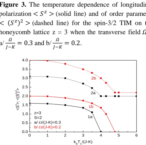
In fig.3, fig.4 and fig.5 are presented the temperature dependences of the longitudinal polarization the order parameter ( ) and the transverse polarization for the honeycomb lattice z = 3 when the transverse field is fixed at some typical values. This quantities display qualitatively the same behavior as the case of spin-1/2.

Figure 1. The phase diagram of the spin-3/2 transverse Ising model for the honeycomb z = 3, square z = 4 and simple cubic lattices z = 6.

0.0 0.1 0.2 0.3 0.4 0.5 0.6 0.7 0.8

0 1 2 3 4 5 6 7

S=3/2

z=6

z=4

z=3

kB TC

/(

J-K

)

(6)

Figure 2. The phase diagram of the spin-2 transverse Ising model for the honeycomb z = 3, square z = 4 and simple cubic lattices z = 6.

Figure 3. The temperature dependence of longitudinal polarization (solid line) and of order parameter

( ) (dashed line) for the spin-3/2 TIM on the honeycomb lattice z = 3 when the transverse field is

a/

and b/ .

Figure 4. The temperature dependence of longitudinal polarization (solid line) and of order parameter

( ) (dashed line) for the spin-2 TIM on the

honeycomb lattice z = 3 when the transverse field is

a/

and b/ .

Figure 5. The temperature dependence of the transverse palarization for spin-3/2 (solid line) and spin-2 (dashed line ) for the honeycomb lattice z=3 for different

values of the transverse field a/

and b/

.

( )

K/J S=3/2 S=2

0.00 12.34 17.98

0.10 9.12 14.01

0.20 6.28 11.34

0.25 4.56 7.87

0,30 1.78 3.67

Table II. The values of the critical transverse field for different values of K for the honeycomb lattice z = 3. At Table II is numerically calculated the critical temperature of the phase transition for different values of correlated tunneling interaction K. It is clear when K increases the temperature of phase transition decreases. There is a critical value KC above which the

phase transition is not observed. When the value of S

and the number of the nearest neighbours increase the

KC increases too. For instance for honeycomb lattice z =

3, for S = 3/2 KC/J = 0.456 and for S = 2 KC/J = 0.629;

for cubic latice z= 4, , for S = 3/2 KC/J = 0.497 and for S

= 2 KC/J = 0.703.

These numerical calculations clearly demonstrate the utility of the Green’s functions of using the method of Tserkovnikov which is appropriate for the spin problems.

0.0 0.2 0.4 0.6 0.8 1.0

0 2 4 6 8

10 S=2

z=6

z=4

z=3

kB TC

/(

J-K

)

/(J-K)

0.0 0.4 0.8 1.2 1.6 2.0 2.4 2.8 3.2 3.6 0.0

0.4 0.8 1.2 1.6 2.0 2.4

z=3 S=3/2 a/ /(J-K)=0.3 b/ /(J-K)=0.2

2b

2a

1b

1a

<S

z >;

<(

S

z ) 2 >

k_BT_C/(J-K)

0 1 2 3 4 5 6

0.0 0.5 1.0 1.5 2.0 2.5 3.0 3.5 4.0

z=3 S=2 a/ /(J-K)=0.3

b/ /(J-K)=0.2

2b

2a

1b

1a

<S

z>;

<(

S

z) 2>

kBTC/(J-K)

0 1 2 3 4 5

0.4 0.6 0.8 1.0 1.2 1.4

z=3 1/ S=3/2

2/ S=2 2b

2a

1b

1a

<

S

x >

(7)

IV. CONCLUSION

We have presented new approximation to treat the TIM system on the base of retarded Green’s functions and method proposed by Tserkovnikov [25] for arbitrary spin S > 1/2. The self- consistent equations obtained are solved and the equilibrium properties of the system a discussed. Because of analytical results, this work will probably have a wider applicability than others methods, especially when one wants to get the temperature dependence in a wide interval of electric properties in the TIM with arbitrary spin. Because of the mathematical simplicity and versatility of our formulation, this method will be very useful for studying and understanding a more complicated physical system like the multiferroics. To our knowledge, the study of TIM with the above method is given for the first time.

V. REFERENCES

[1] R. Blinc and B.Zeks, Soft mode in Ferroelectrics and Antiferroelectrics, (North-Hoilland, Amsterdam, 1974).

[2] R. B. Stinchcombe, J. Phys. C: Solid St. Phys. 6, 2459 (1973).

[3] A. Kuehnel, S. Wendt, and J. Wesselinowa, Phys. stat. sol. (b) 84, 653 (1977).

[4] B. H. Teng and H. K. Sy, Europhys. Lett. 73, 601 (2006).

[5] S. J. Oitmaa and G. J. Coombs, J. Phys. C 14, 143 (1981).

[6] S. Y. Ma and C. Gong, J. Phys.: Condens. Matter 4, L313 (1992).

[7] S. T. Kaneyoshi, M. Jascur and I. P. Fittipaldi, Phys. Rev. B 48, 250 (1993).

[8] S. A. Elkouraychi, M. Saber and J. W. Tucker, Physica A 213, 576 (1995).

[9] J. Strecka and M. Jascur, acta phys. slov. 65, 235 (2015).

[10] E. B. Brown, Phys. Rev. B 43, 13664 (1991). [11] M. Fiebig, J. Phys. D: Appl. Phys. 38, R123

(2005).

[12] H. Wu, Q. Jiang, and W. Z. Shen, Phys. Lett. A 330, 358 (2004).

[13] T. Michael and S. Trimper, Phys. Rev. B 83, 134409 (2011).

[14] Y. Liu, L.-J. Zhai and H.-Y. Wang, Chin. Phys. B 24, 037510 (2015).

[15] J. Wesselinowa and I. Apostolova, J. Appl. Phys. 104, 084108 (2008).

[16] J. M. Wesselinowa and St. Kovachev, J. Appl. Phys. 102, 043911 (2007).

[17] S. G. Bahoosh, J. M. Wesselinowa and S. Trimper, phys. stat. sol. (b) 250, 1816 (2013). [18] Z. Wang and M. J. Grimson, Eur. Phys. J. Appl.

Phys. 70, 30303 (2015).

[19] B. B. Van Aken, T. T. M. Palstra, A. Filippetti and N. A. Spaldin, Nat.Mater. 3, 164 (2004). [20] A. Inomata and K. Kohn, J. Phys.: Condens.

Matter 8, 2673 (1996).

[21] F. Zavaliche, S. Y. Yang, T. Zhao, Y. H. Chu, M. P. Cruz, C. B. Eom and R. Ramesh, Phase Transitions 79, 991 (2006)).

[22] F. Zavaliche, R. R. Das, D. M. Kim, C. B. Eom, S. Y. Yang, P. Shafer and R. Ramesh, Appl. Phys. Lett. 87, 182912 (2005).

[23] C. Michel, J.-M. Moreau, G. D. Achenbechi, R. Gerson and W. J. James, Solid State Commun. 7, 701 (1969).

[24] S. K. Streiffer, C. B. Parker, A. E. Romanov, M. J. Lefevre, L. Zhao, J. S. Speck, W. Pompe, C. M. Foster and G. R. Baiet, J. Appl. Phys. 83, 2742 (1998).

[25] Yu. A. Tserkovnikov, Theor. Math. Fiz. 7, 250 (1971).