COVERAGE VS NODE & DEPLOYMENT CHARACTERISTICS FOR WIRELESS SENSOR NETWORKS

COVERAGE VS NODE & DEPLOYMENT

CHARACTERISTICS FOR WIRELESS SENSOR

NETWORKS

Vishal Gupta

, M.N.Doja

1

Research Scholar, 2Professor, Department of Computer Engineering, JMI, Delhi, (India)

ABSTRACT

Coverage is a very important parameter because it measures how effectively a target field is monitored by the

sensor network. This paper provides a comparative statistics for the impact of various node characteristics on

the area coverage. In this paper, we have also focused on sensor networks with two types of nodes that differ in

their capabilities, and discussed the effects of heterogeneity of sensing on the network coverage. This work can

serve as a guideline for designing large-scale sensor networks cost-effectively. The work can also be extended to

more complicated heterogeneous wireless sensor networks with more than two types of sensors.

Keywords: Coverage, Heterogeneity, Wireless Sensor Network (WSN)

I. INTRODUCTION

Sensing coverage is one of the fundamental QoS problems in sensor networks is sensing coverage. Coverage in

sensor networks is a measure to how closely target area is observed by the sensor nodes. The coverage problem

in sensor networks was first investigated as one of the network QoS metrics by Meguerdichian et al. [1]. Due to

the resource constraint nature of the sensor node/WSN, there are many limitations in this area. [2] Provides

some details about the sensor nodes with respective processing capabilities.

Intuitively, it seems that the introduction of some sensor nodes with greater capabilities can help enhance the

overall network coverage. However questions of whether how many and what types of heterogeneous resources

to deploy remain largely unexplored [3]. This raises the issue of quantifying the effects of deploying

heterogeneous sensor nodes on the quality of service (QoS) of the whole network.

The rest of the paper is organized as follows. Section II gives the definition of coverage and its types. Section

III, provides the brief survey of some the research done in this area. In section IV, we have presented our work

with the simulation support in MatLab. Finally, fifth section gives a summary and the conclusion of the paper.

II. COVERAGE

According to [4], in the given sensor network, coverage denoted by C is defined as the mapping from a set of

sensors S, to the set of area A, in the given field of interest F or Coverage C is defined as a mapping C:S→A

such that ∀si∈S, ∃ai∈A and overlapping between each ai is removed, where:

2. A is the set of area denoted by ai which is identified by summing π*(Rsi)2, where Rsi is the sensing radius of

sensor si.

3.F is the given area which has to be monitored (Field of Interest).

4. C is termed as coverage which maps S to A.

5. Cardinality of S and A are same.

To be specific, it reflects how well the sensed field is monitored or tracked by the sensors.

Depending upon the objectives and applications, three types of coverage are defined in the literature

[5][6][7][8]: Area Coverage: To ensure that every point of the whole area to be monitored by at least one sensor

node. Point/Target Coverage: To cover up the set of predetermined target/s in the given region of interest

(ROI).

Barrier Coverage: To guarantee that every object moving across the given barrier to be detected by the

deployed sensors.

The problem of area coverage deals with two important factors: the node type and the deployment strategy.

Node can be of different types: static, dynamic, homogeneous and heterogeneous. The deployment strategy can

be: Deterministic, Random, Sparse or Dense. The selection of proper node and deployment strategy depends on

the application in which sensor nodes are going to be used.

III. LITERATURE REVIEW

Authors in [9] have discussed different types of coverage issues. Full coverage issue is examined by considering

different points such along with the strategy used to detect full coverage and positioning based/independent

algorithms.

In paper [10], the authors have established the optimal polynomial time algorithm in worst-case and

average-case for network coverage calculation using graph theoretic and computational geometry. C. M. Cardei et al. [7]

have suggested one method to improve the sensor network lifetime while providing target point coverage using

the concept of set covers.

A. Chen et al. in [8] have proposed a Localized Barrier Coverage Protocol (LBCP). P. Balister et al. in [11]

suggested a method to find reliable density estimates for providing barrier coverage in belt shaped region and

connectivity in network.

In [12] Maxim A. Batalin et al., have used a mobile robot to traverse and deploy sensor nodes in the given target

area. Saurabh Ganeriwal et al. [13] proposed an algorithm to repair coverage gap due to reduction in energy of

sensor node.

Ziqiu Yun et al. [14] have studied different arrangements for sensor deployment to provide full coverage and

k-connectivity (K<6). Work of S. A. R. Zaidi et al. [15] gives solution to the problem of providing full coverage in

target field with minimum number of sensors for any geometrical area in case of deterministic deployment.

[16] Discusses the impact of Heterogeneity on Coverage and Broadcast Reachability in Wireless Sensor

Networks. M Singaram et al. [17] proposed ERGS algorithm for randomly deployed sensor nodes. Optimal

Geographical Density Control (OGDC) algorithm by H. Zhang et al. [18] considers dense deployment for

sensors in the monitoring area. In [19] the authors have proposed a circle intersection localized coverage

This work is an extension of our earlier work [20] that dealt with the trade-off between number of sensor nodes

deployed and coverage in WSN.

IV. PROPOSED WORK

In this work, we have simulated the change in the coverage obtained by varying the node and deployment

characteristics. In all cases, we have assumed the static node, random deployment strategy. The complete work

can be divided into following cases. A very large number of iterations have been taken to derive at the result and

conclusion in every case.

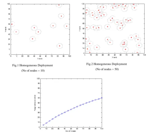
4.1 Homogeneous Deployment Case

4.1.1 Effect on the coverage from sparse to dense deployment keeping sensing range constant.

Area = 100 * 100 unit Sensing Range = 5 unit (constant)

Fig.1 Homogeneous Deployment

(No of nodes = 10)

Fig.2 Homogeneous Deployment

(No of nodes = 50)

Result: As shown by the graph in Fig.3, increasing the number of nodes deployed in ROI doesn’t result in the

proportionate increase in the coverage area.

4.1.2 Effect on the coverage with respect to the change in the sensing range of the nodes keeping number

of nodes constant.

Area = 100 * 100 unit Number of Nodes = 20 (Constant)

Fig.4 Homogeneous Deployment

(Sensing range = 5 Unit)

Fig.5 Homogeneous Deployment

(Sensing range = 10 Unit)

Fig. 6 Homogeneous Deployment (%Coverage Vs Sensing Range of the Nodes)

Result: As shown by the graph in Fig.6, increasing the sensing range of the deployed nodes directly affects the

coverage gain initially in the ROI. But beyond a point, this increase has virtually no effect on the coverage as

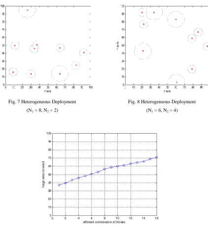
4.2 Heterogeneous Deployment Case

4.2.1 Effect on the coverage keeping number of nodes constant.

Area = 100 * 100 unit, No of Nodes = 10 (Constant),

SR1 = 5 Unit, SR2 = 10 Unit

Fig. 7 Heterogeneous Deployment

(N1 = 8, N2 = 2)

Fig. 8 Heterogeneous Deployment

(N1 = 6, N2 = 4)

Fig. 9 Heterogeneous Deployment

(%Coverage Vs Different combinations of nodes keeping total number of nodes constant)

(SR1 = 10, SR2 =20, No of nodes = 15)

Result: As shown by the graph in Fig.9, increasing the number of nodes with higher sensing range in the mix

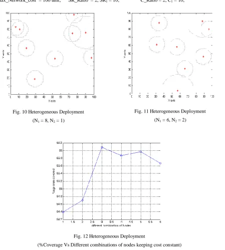
4.2.2 Effect on the coverage keeping the cost of the network constant.

Max_Network_cost = 100 unit; SR_Ratio = 2; SR1 = 10; C_Ratio = 2; C1 = 10;

Fig. 10 Heterogeneous Deployment

(N1 = 8, N2 = 1)

Fig. 11 Heterogeneous Deployment

(N1 = 6, N2 = 2)

Fig. 12 Heterogeneous Deployment

(%Coverage Vs Different combinations of nodes keeping cost constant)

(Max_Network_cost = 200; SR_Ratio = 2; SR1 = 20; C_Ratio = 2; C1 = 20;)

Result: As shown by the graph in Fig.12, increasing the number of nodes with higher sensing range in the mix

keeping cost to the network constant increases the coverage area. But the graph shows a strange behaviour that

going beyond a range; the result may have adverse effect.

V. CONCLUSIONS

Coverage is a basic issue in wireless sensor networks. In this paper, the coverage issue was discussed. Area

We conclude that for homogenous networks, enhancing the node characteristics doesn’t necessary increase the

coverage in the same proportion. This is due to the increase in the overlapping of the area covered by different

nodes. Similarly, for heterogeneous networks, increasing the high quality nodes in comparison to the low quality

nodes does not necessarily qualify for the improved coverage area. Again the reason is the overlapping that

seems to have more negative effects when the high quality nodes get increasing in number as compared to low

quality nodes.

We further conclude that the heterogeneity may give improved results when the deployment is deterministic as

the high quality & hence the costly nodes may be placed at appropriate points in the ROI for maximum

coverage.

In this work, we have not considered the environment that may have obstacles through which radio signals

cannot propagate.

REFERENCES

[1]. S. Meguerdichian, F. Koushanfar, M. Potkoljak and M. B. Srivastava, "Coverage problems in wireless

ad-hoc sensor networks", Twentieth Annual Joint Conference of the IEEE Computer and

Communications Societies (INFOCOM 2001), vol. 3, April, 22-26 2001, pp. 1380 - 1387.

[2]. “List of wireless sensor nodes” main page en.wikipedia.org, [Online] Available at: ht

tp://en.wikipedia.org/wiki/List of wireless sensor nodes

[3]. M. Yarvis, N. Kushalnagar, H. Singh, A. Rangarajan, Y Liu, and S. Singh, "Exploiting heterogeneity in

sensor networks," Proc. of IEEE INFOCOM, 2005.

[4]. C. Zhu, C. Zheng, L. Shu and G. Han, “A survey on coverage and connectivity issues in wireless sensor networks”, Journal of Network and Computer Applications, Volume 35, Issue 2, March 2012, Pages

619-632.

[5]. R. Mulligan, H. M. Ammari, “Coverage in Wireless Sensor Networks”, Network Protocols and

Algorithms, ISSN 1943-3581, 2010, Vol. 2, No. 2.

[6]. L. Mo, L. Zhenjiang and A.V. Vasilakos, “A Survey on Topology Control in Wireless Sensor Networks:

Taxonomy, Comparative Study, and Open Issues”, Proc. of the IEEE, vol.101, no.12, pp.2538-2557,

Dec.2013

[7]. M. Cardei, M. T. Thai, Li Yingshu and W. Weili, “Energy-efficient target coverage in wireless sensor networks”, 24th Annual Joint Conference of the IEEE Computer and Communications Societies

INFOCOM 2005. Proceedings IEEE, vol.3, pp.1976-1984, 13-17 March 2005.

[8]. A. Chen, S. Kumar, and T. H. Lai, “Designing localized algorithms for barrier coverage”, Proc. of the

13th annual ACM international conference on Mobile computing and networking (MobiCom ’07), ACM,

New York, NY, USA, 2007, 63 -74

[9]. A. Singh and T. P. Sharma, “A survey on area coverage in wireless sensor networks”, International

Conference on Control, Instrumentation, Communication and Computational Technologies (ICCICCT),

[10]. S. Megerian, F Koushanfar, M. Potkonjak, and M. B. Srivastava, "Worst and best-case coverage in

sensor networks", IEEE Transactions on Mobile Computing, vol. 4, no. 1, pp. 84-92, January/February

2005.

[11]. P. Balister, B. Bollobas, A. Sarkar, and S. Kumar, “Reliable density estimates for coverage and

connectivity in thin strips of finite length”, Proc. of the 13th annual ACM international conference on

Mobile computing and networking (MobiCom ’07), ACM, New York, NY, USA, 2007, 75-86

[12]. M. A. Batalin and G. S. Sukhatme, “Coverage, exploration, and deployment by a mobile robot and communication network”, Proc. of the 2nd international conference on Information processing in sensor

networks, Springer-Verlag, Berlin, Heidelberg, 2003, 376-391.

[13]. S. Ganeriwal, A. Kansal and M.B. Srivastava, “Self aware actuation for fault repair in sensor networks”,

Proc. of IEEE International Conference on Robotics and Automation (ICRA ’04), vol.5, pp.5244-5249,

April 26 2004-May 1 2004

[14]. Y. Ziqiu, B. Xiaole, X. Dong, T .H Lai and J. Weijia, “Optimal Deployment Patterns for Full Coverage

and k -Connectivity (k ≤ 6) Wireless Sensor Networks”, IEEE/ACM Transactions on Networking

,vol.18, no.3, pp.934-947, June 2010

[15]. S. A. R. Zaidi, M. Hafeez, S.A. Khayam, D.C. McLernon, M. Ghogho and K. Kim, “On minimum cost coverage in wireless sensor networks”, 43rd Annual Conference on Information Sciences and Systems

(ACISS 2009) pp.213-218, 18-20 March 2009

[16]. Y. Wang, X. Wang, D. P. Agrawal and A. A. Minai, “Impact of Heterogeneity on Coverage and

Broadcast Reachability in Wireless Sensor Networks”, Proc. of 15th International Conference on

Computer Communications and Networks, (ICCCN 2006) 2006. Pages: 63

67, DOI: 10.1109/ICCCN.2006.286246

[17]. M. Singaram, S. Finney, D. Shadrach, N. S. Kumar and V. Chandraprasad, “Energy Efficient Self-Scheduling Algorithm for Wireless Sensor Networks”, International Journal of Scientific and Technology

Research Volume 3, Issue 1, January 2014.

[18]. H. Zhang and J. C. Hou, “Maintaining Sensing Coverage and Connectivity in Large Sensor Networks”, in

Ad Hoc and Sensor Wireless Networks, Vol. 1, 3 March 2005, pp. 89-124

[19]. H. Xin, Y. Ke and G. Xiaolin, “The Area Coverage Algorithm to Maintain Connectivity for WSN”, Ninth

IEEE International Conference on Computer and Information Technology, 2009. CIT '09, Year:

2009, Volume: 2, Pages: 81 - 86, DOI: 10.1109/CIT.2009.82

[20]. G. Bhatia, V. Gupta and M. N. Doja, “Trade off between number of sensor nodes deployed and coverage in WSN”, International Journal of Engineering Technology, Management and Applied Sciences, Vol. 2