Maryam et al. World Journal of Engineering Research and Technology
A REVIEW ON DIMENSIONALITY REDUCTION USING COPULA
APPROACH IN DATA MINING
Sumaiya Maryam* and Sriram Yadav
M.Tech. Scholar, MITS, Bhopal.
A.P., CSE, MITS Bhopal.
Article Received on 18/08/2019 Article Revised on 08/09/2019 Article Accepted on 29/09/2019
ABSTRACT
Copula approach is a Sampling-based dimensionality reduction
technique. Removing linearly redundant combined dimensions, giving
a convenient way to generate correlated multivariate random variables.
Managing the integrity of the original information, deducting the dimension of data space
without losing valuable information. The modern trends in collecting very large and diverse
datasets have created a great challenge in data analysis. The recent trends in collecting very
large and diverse datasets have created a great challenge in data analysis. One of the
attributes of these gigantic datasets is that they often have significant amounts of
redundancies. The use of very large multi-dimensional data will result in more noise,
redundant data, and the possibility of unconnected data entities. To efficiently manage data
represented in a high-dimensional space and to address the impact of redundant dimensions
on the final results, a new technique has been proposed for the dimensionality reduction using
Copulas and the LU-decomposition (Forward Substitution) method. The proposed method is
compared favorably with existing approaches on real-world datasets: Diabetes, Waveform,
two versions of Human Activity Recognition based on Smartphone, and Thyroid Datasets
taken from machine learning repository in terms of dimensionality reduction and efficiency
of the method, which are performed on statistical and classification measures.
KEYWORDS: Data mining, Integrity, Sampling, Copulas, Dimensionality reduction, Redundancy, LU-Decomposition.
World Journal of Engineering Research and Technology
WJERT
www.wjert.org
SJIF Impact Factor: 5.924*Corresponding Author
Sumaiya Maryam
M.Tech. Scholar, MITS,
INTRODUCTION
Dimensionality reduction technique is based on probabilistic and sampling models; therefore,
one needs to recall some fundamental concepts. These include the notions of a Probability
Density Function (PDF), Cumulative Distribution Function (CDF), a random variable used to
generate samples from a probability distribution, a Copula to model dependencies of data
without imposing constraints to specific types of marginal probability density functions, and
dependence and rank correlations of multivariate random variables to measure dependencies
of the dimensions.
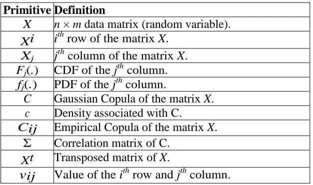
The following table gives basic notations used throughout this paper
Table 1: Basic notations.
Primitive Definition
X n × m data matrix (random variable). Xi ithrow of the matrix X.
Xj jthcolumn of the matrix X. Fj(.) CDF of the jthcolumn.
fj(.) PDF of the jthcolumn.
C Gaussian Copula of the matrix X.
c Density associated with C.
Cij Empirical Copula of the matrix X.
Σ Correlation matrix of C.
Xt Transposed matrix of X.
vij Value of the ithrow and jthcolumn.
Let f be the Probability Density Function (PDF) of a random variable X. The probability
distribution of X consists in calculating the probability P(X1 ≤ x1, X2 ≤ x2,……Xm ≤ xm),
for all(X1,……,Xm) belongs to Rm. It is completely specified by the CDF F which is defined
in (Rubinstein &Kroese, 2011) as follows:
F(x1, x2,….., xm) = P(X1 ≤ x1,X2 ≤ x2,…., m ≤ xm) ---(1)
1.1 Random Variable Generation
The problem of generating a sample from a one-dimensional cumulative distribution function
CDF by calculating the inverse transform sampling. To illustrate the problem, let X be a
continuous random variable with a CDF F (x) = P [X≤ x], and U be a continuous uniform
distribution over the interval [0, 1]. The transform X = F −1(U ) denotes the inverse transform
sampling function of a given continuous uniform variable U = F (X) in [0, 1], where F −1(u) =
{min x, F (x) ≥ u } (Rubinstein & Kroese, 2011). So the simple steps used for generating a
1. Generate U ∼ U [0, 1];
2. Return X = F−1 (U).
The usual problem is how to combine one- dimensional distribution functions to form
multivariate distributions and how to estimate and simulate their density f (x1, x2, ..., xm) to
obtain the required number of random samples of Xi, i=1,...,m, especially in high-dimensional
spaces. This problem will be explained in the following section.
1.2 Modeling with Copulas
The first usage of Copulas is to provide a convenient way to generate correlated multivariate
random variable distributions and to present a solution for the difficulties of transformation of
the density estimation problem.
To illustrate the problem of invertible transformations of m-dimensional continuous random
variables X1,..., Xm according to their CDF, into m independently uniformly-distributed
variables U1 = F1(X1), U2 = F2(X2),..., Um = Fm(Xm), let f (x1, x2, ..., xm) be the probability
density function of X1, ..., Xm, and let c(u1, u2, ..., um) be the joint probability density function
of U1, U2, ..., Um. In general, the estimation of the probability density function f (x1, x2,...,
xm) can provide a nonparametric form (unknown families of distributions). In this case, the
probability density function c(u1, u2, ..., um) of U1, U2, ..., Um has been estimated instead of that X1, ...,
Xm to simplify the density estimation problem, and then simulated it to achieve the random
samples X1, ..., Xmusing the inverse transformations Xi= F −1(Ui).
Sklar's Theorem showed that there exists a unique m-dimensional Copula C in [0, 1]m with
standard uniform marginal distributions U1,…..Um. (Nelsen, 2007) states that every
distribution function Fwith margins F1... Fm can be w r i t t e n as:
F (X1, ..., Xm) = C(F1(X1), ..., Fm(Xm))., ∀(X1, ..., Xm) ∈ IRm (2)
To evaluate the suitability of a selected Copula with estimated parameter and to avoid the
introduction of any assumptions on the distribution Fi(Xi), one can utilize an empirical CDF
of a marginal Fi(Xi), to transform m samples of X into m samples of U. An empirical Copula
is useful for examining the dependence structure of m u l t i v a r i a t e random vectors. Formally,
the empirical Copula is given by the following equation:
Where the function I(arg) is the indicator function, which equals 1 if arg is true and 0 otherwise.
Here, m is used to keep the empirical CDF less than 1, where m is the number of
observations. In the following, we will focus on the Copula those results from a standard
multivariate Gaussian Copula.
1.3 Gaussian Copula
The difference between the Gaussian Copula and the joint normal CDF is that the Gaussian
Copula allows having different marginal CDF types from the joint distribution (Nelsen,
2007). However, in probability theory and statistics, the multivariate normal distribution is a
generalization of the one-dimensional normal distribution. The Gaussian Copula is defined as
follows:
C(Ф(x1),….. Ф(xm)) = 1/ exp(-1/2 Xt(Σ−1−I)X ) (4)
Where Φ (xi) is the CDF standard Gaussian distribution of fi (xi), i.e., Xi ∼N (0, 1), and Σ is the
correlation matrix. The resulting Copula C(u1, ..., um) is called Gaussian Copula. The density
associated with C(u1, ..., um) is obtained with the following equation:
C (u1,…., um) =1/ exp[-1/2 ] (5)
Where ui =Ф(xi), and ξ = (Φ−1(u1),………., Φ−1(um))T.
1.4 Dependence and Rank Correlation
Since the Copula of a multivariate distribution describes its dependence structure, it might
be appropriate to use measures of dependence which are Copula-based. The Pearson
correlation measures the relationship Σ = cov(Xi, Xj)/(σXi σXj ) where cov(Xi, Xj) is the
covariance of Xi and Xj while σXi , σXj are the standard deviations of Xi and Xj. Kendall
rank correlation (also known as Kendall’s coefficient of concordance) is a non- parametric
test that measures the strength of dependence between two random samples Xip ;Xip of n
observations. The notion of concordance can be defined by the following equation:
τ = P [(Xi − Xj) (Xit − Xj) > 0] –P [(Xi− Xj) (Xit − Xj) <0] (6)
2. LITERATURE REVIEW
2.1 Linear dimensionality reduction
Principal Component Analysis (PCA) is a well established method for dimensionality
reduction. It derives new variables (in decreasing order of importance) that are linked by
linear combinations of the original variables and are uncorrelated. Several models and
techniques for data reduction based on PCA have been proposed (Sasikala & Balamuru- gan,
2013). (Zhai et al., 2014) proposed a maximum likelihood approach to the multi-size PCA
problem. The covariance based approach was ex- tended to estimate errors within the
resulting PCA decomposition. Instead of making all the vectors of fixed size and then
computing a covariance matrix, they directly estimate the covariance matrix from the
multi-sized data using nonlinear optimization. (Kerdprasop et al., 2014) studied the recognition
accuracy and the execution times of two different statistical dimensionality reduction methods
applied to the biometric image data, which are: PCA and Linear Discriminat Aanalysis
(LDA). The learning algorithm that has been used to train and recognize the images is a support
vector machine with linear and polynomial kernel functions. The main drawback of reducing
dimensionality with PCA is that it can only be used if the original variables are correlated, and
homogeneous, if each component is guaranteed to be independent and if the dataset is
normally distributed. If the original variables are not normalized, PCA is not effective.
The Sparse Principal Component Analysis (SPCA) (Zou et al., 2006) is an improvement of the
classical method of PCA to overcome the problem of correlated variables using the LASSO
technique. LASSO is a promising variable selection technique, producing accurate and sparse
models. SPCA is based on the fact that PCA can be written as a regression problem where the
response is predicted by a linear combination of the predictors. There- fore, a large number of
coefficients of principal components become zero, leading to a modified PCA with sparse
loading. Many studies on data reduct- tion based on SPCA have been presented. (Shen &
Huang, 2008) proposed an iterative algorithm named sparse PCA via regularized SVD
(sPCA- rSVD) that uses the close connection between PCA and singular value decomposition
(SVD) of the data matrix and extracts the PCs through solving a low rank matrix
approximation problem. (Bai et al., 2015) proposed a method based on sparse principal
component analysis for finding an effective sparse feature principal component (PC) of
multiple physiological signals. This method identifies an active index set corresponding to the
× × ×
× ×
× × ×
Singular Value Decomposition (SVD) is a powerful technique for dimensionality reduction. It
is a particular case of the matrix factorization approach and it is therefore also related to PCA.
The key is- sue of an SVD decomposition is to find a lower dimensional feature space by
using the matrix product U S V , where U and V are two orthogonal matrices and S is a
diagonal matrix with m × m, m ×n, and n× n dimensions, respectively. SVD retains only r× n
positive singular values of low effect to reduce the data, and thus S becomes a diagonal
matrix with only r non-zero positive en- tries, which reduces the dimensions of these three
matrices to m × r, r× r, and r× n, respectively. Many studies on data reduction have been
presented which are built upon SVD, such as the ones used in (Zhang et al., 2010) and
(Watcharapinchai et al., 2009). (Lin et al., 2014) developed a dimensionality reduction
approach by applying the sparsified singular value decomposition (SSVD). Their paper
demonstrates how SSVD can be used to identify and remove nonessential features in order to
facilitate the feature selection phase, to analyze the application limitations and the
computational complexity. However, the application of SSVD on large datasets showed a loss
of accuracy and makes it difficult to compute the eigenvalue decomposition of a matrix product
AT A, where A is the matrix of the original data.
2.2 Nonlinear dimensionality reduction
A vast literature devoted to nonlinear techniques has been proposed to resolve the problem of
dimensionality reduction, such as manifold learning methods, e.g., Locally Linear Embedding
(LLE), Isometric mapping (Isomap), Kernel PCA (KPCA), Laplacian Eigenmaps (LE), and a
review of these methods is summarized in (Gisbrecht & Hammer, 2015; Wan et al., 2016).
KPCA (Kuang et al., 2015) is a nonlinear generalization of PCA in a high-dimensional kernel
space constructed using kernel functions. By comparing with PCA, KPCA computes the
principal eigenvectors using the kernel matrix, rather than the covariance matrix. A kernel
matrix is done by computing the inner product of the data points. LLE (Hettiarachchi &
Peters, 2015) is a nonlinear dimensionality reduction technique based on simple geometric in-
tuitions. This algebraic approach computes the low-dimensional neighborhood preserving
embeddings. The neighborhood is preserved in the embedding based on a minimizing cost
function in input space and output space, respectively. Isomap (Zhang et al., 2016) explores
an underlying manifold structure of a dataset based on the computation of geodesic manifold
distances between all pairs of data points. The geodesic distance is determined as the length of
the shortest path along the surface of the manifold between two data points. It first constructs
neighbors in the input space. Then, it estimates geodesic distances of all pairs of points by
calculating the shortest path distances in the neighborhood graph. Finally, multidimensional
scaling (MDS) is applied to the arising geodesic distance matrix to find a set of
low-dimensional points that greatly match such distances.
2.3 Sampling dimensionality reduction
Other widely used techniques are based on sampling. They are used for selecting a
representative subset of relevant data from a large dataset. In many cases, sampling is very
useful because processing the entire dataset is computationally too expensive. In general, the
critical issue of these strategies is the selection of a limited but representative sample from
the entire dataset. Various random, deterministic, density biased sampling, pseudo-random
number generator and sampling from non-uniform distribution strategies exist in the literature
(Rubinstein & Kroese, 2011). How- ever, very little work has been done on the Pseudo-
random number generator and sampling from non- uniform distribution strategies, especially
in the multi-dimensional case with heterogeneous data. Naive sampling methods are not
suitable for noisy data which are part of real-world applications, since the performance of the
algorithms may vary un- predictably and significantly. The random sampling approach
effectively ignores all the information present in the samples which are not part of the reduced
subset (Whelan et al., 2010). An advanced data reduction algorithm should be developed in
multi-dimensional real-world datasets, taking into account the heterogeneous aspect of the
data. Both approaches (Colom´e et al., 2014)(Fakoor & Huber, 2012) are based on sampling and
a probabilistic representation from uniform distribution strategies. The authors of (Fakoor &
Huber, 2012) pro- posed a method to reduce the complexity of solving Partially Observable
Markov Decision Processes (POMDP) in continuous state spaces. The paper uses sampling
techniques to reduce the complexity of the POMDPs by reducing the number of state
variables on the basis of samples drawn from these distributions by means of a Monte Carlo
approach and conditional distributions. The authors in (Colom´e et al., 2014) applied
dimensionality reduction to a recent movement representation used in robotics, called
Probabilistic Movement Primitives (ProMP), and they addressed the problem of fitting a
low-dimensional, probabilistic representation to a set of demonstrations of a task. The authors
fitted the trajectory distributions and estimated the parameters with a model-based stochastic
using the maximum likelihood method. This method assumes that the data follow a
multivariate normal distribution which is different from the typical assumptions about the
results for different assumptions about the data distribution and estimate the optimal space
dimension of the data.
2.4 Similarity measure dimensionality reduction
There are other widely used methods for data reduction based on similarity measures
(Wencheng,2010)(Pirolla et al., 2012) (Zhang et al., 2010). Ac- cording to (Dash et al., 2015),
the presence of redundant or noisy features degrades the classification performance, requires
huge memory, and consumes more computational time. (Dash et al., 2015) proposes a
three-stage dimensionality reduction technique for microarray data classification using a comparative
study of four different classifiers, multiple linear regression (MLR), artificial neural network
(ANN), k-nearest neighbor (k-NN), and naive Bayesian classifier to observe the improvement
in performance. In their experiments, the authors reduce the dimension without compromising
the performance of such models. (Deegalla et al., 2012) proposed a dimensionality reduction
method that employs s classification approaches based on the k-nearest neighbor rule. The
effectiveness of the reduced set is measured in terms of the classification accuracy. This
method attempts to derive a minimal consistent set, i.e., a minimal set which correctly
classifies all the original samples (Whelan et al., 2010). (Venugopalan et al., 2014) discussed
the ongoing work in the field of pattern analysis for bio-medical signals (cardio-synchronous
waveform) using a Radio Frequency Impedance Interrogation (RFII) device for the purpose of
user identification. They discussed the feasibility of reducing the dimensions of these signals
by projecting them into various sub-spaces while still preserving inter-user discriminating
information, and they compared the classification performance using traditional dimensionality
reduction methods such as PCA, independent component analysis (ICA), random projections,
or k-SVD-based dictionary learning. In the majority of cases, the authors see that the space
obtained based on classification carries merit due the dual advantages of reduced dimension
and high classification.
Developing effective clustering methods for high- dimensional datasets is a challenging task
(Whelan et al., 2010). (Boutsidis et al., 2015) studied the topic of dimensionality reduction
for k-means clustering that encompasses the union of two approaches: 1) A feature
selection-based algorithm selects a small subset of the input features and then the k-means is applied on
the selected features. 2) A feature extraction-based algorithm constructs a small set of new
artificial features and then the k- means is applied on the constructed features. The first
approximate SVD factorization. (Sun et al., 2014) developed a tensor factorization based on a
clustering algorithm (k-mean), referred to as Dimensionality Reduction Assisted Tensor
Clustering (DRATC). In this algorithm, the tensor decomposition is used as a way to learn
low-dimensional representation of the given tensors and, simultaneously, clustering is con- ducted by
coupling the approximation and learning constraints, leading to the PCA Tensor Clustering
and Non-negative Tensor Clustering models.
Problems identification and Objectives
The most serious problem is the presence of missing values in datasets. Missing values can
result in loss of efficiency of the dimensionality reduction approach, lead to complications in
handling and analyzing the data, or distort the relationship between the data distribution.
Also, it is interesting to investigate the possibility of using Meta heuristics or hybrid
approaches to determine a solution of the proposed optimization problem in the Big Data
setting. Objectives of the research work are to overcome several problems identified and strong
efforts to improve the performance of the dimensionality reduction approach in very large
datasets.
Proposed Methodology
The approach presented in this paper for dimensionality reduction in very large datasets is
based on the theory of Copulas and the LU-decomposition method (Forward Substitution). The
main goal of the method is to reduce the dimensional spaces of data without losing
important/interesting information. On the other hand, the goal is to estimate the multivariate
joint probability distribution without imposing constraints on specific types of marginal
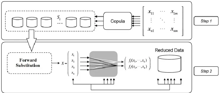
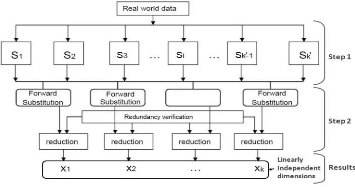
distributions of dimensions. Figure 1 shows an overview of the proposed reduction method
which operates in two main steps.
In the first step, large raw datasets are decomposed into smaller subsets when calculating the
data dependencies using a Copula by taking into account heterogeneous data and removing the
data which are strongly dependent. In the second step, we want to reduce the space
dimensions by eliminating dimensions that are linear combinations of others. Then we will
find the coefficients of the linear combination of dimensions by applying the
LU-decomposition method (Forward Substitution) to each subset to obtain an independent set of
variables in order to improve the efficiency of data mining algorithms. The two different steps
of the pro- posed method are as follows (See also Figure 1):
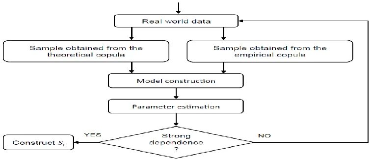
Step 1: Construction of dependent sample subset Si, (i=1,...,kt)
In order to decompose the real-world dataset into smaller dependent sample subsets, vectors
are considered which are linearly dependent in the original data.
Empirical Copula will be calculated first to better observe the dependencies between
variables. According to the marginal distributions from the observed and approved empirical
Copula, we can determine the theoretical.
Figure 2: Construction of the subsets Si, (i=1,...,kt).
Copula, that links univariate marginal distributions to their joint multivariate distribution
function, and then we will regroup dimensions having the strong correlation relationship in
each sample subset Si,(i=1,...,kt) by estimating the parameters of the Copula. In this paper, we
have presented the Gaussian Copula that corresponds to our experimental results. An
illustration of the Copula method is given in Figure 2.
The dependence between two continuous random variables X1 and X2 is defined as follows: If
×
meaning that the values of X1 increase as the values of X2 increase (i.e., the more each at-
tribute implies the other). Hence, a higher value may indicate that X1 and X2 are positively
dependent, and probably have a highly redundant attribute, then these two samples will be
made as in the same subset Si,(i=1,...,kt). When the parameter of the Copula ρ of the two
continuous random variables X1 and X2 is greater than 0.7, then X1 and X2 have a strong
dependence. If the resulting value is equal or less than 0, then X1 and X2 are independent and
there is no correlation between them.
The output of the sample subset Si,(i=1,...,kt) represents a matrix that retains only dependent
samples of the original matrix in order to detect, and remove a maximum of the redundant
dimensions, which are linear combinations of others, in the second step.
Step 2: LU-decomposition method
The key idea behind the use of the Forward Substitution method is to solve the linear system
equations as given by the samples Si,(i=1,...,kt) with an upper-triangular coefficient matrix in
order to find the coefficients of linear sample combinations and to provide a low linear space
(Xi;i=1,……k) of the original matrix as shown in Figure 3.
Figure 3: Schema of dimensionality reduction.
The LU decomposition method is an efficient procedure for solving a system of linear
equations αχ S´ = C, and it can help accelerate the computation. When C is a column vector in
the dependent sample subsets Si,(i=1,...,kt), and αj is an output vector representing the
SSi;(i=1,….k’-1) induces a lower triangular matrix without column C. We conclude that each
matrix S´i,(i=1,...,kt−1) induces a lower triangular matrix of the following form:
(‘S) {α1x11 = c1
{α1x21 + α2x22 = c2 (8)
{α1xn1 + α2xn2 + ... + αnxnn = cn
From the above equations, we see that α1 = c1/x11. Thus, we compute α1 from the first
equation and substitute it into the second to compute α2,..., etc. Repeating this process, we
reach equation i, 2≤ i ≤n, using the following formula:
αi = 1/xi[ci- ], i=2,,,n (9)
Algorithm 1: Dimensionality linear combination reduction method
Input: Vector C and a lower triangular matrix ‘S; Output: Vector α.
Begin
α1 = c1/x11
for i := 2 to n do
αi = ci
for j := 1 to i -1 do
αi=αi - xijαj
end
αi = αi/xii
end
The algorithm 1 used for this resolution makes (n × (n - 1))/2 additions and subtractions, (n×
(n - 1))/2 multiplications and n divisions to calculate the solution, a global number of
operations in the order of n2.
CONCLUSIONS
In this paper, we have proposed a new method for dimensionality reduction in the data
pre-processing phase of mining high-dimensional data. This ap proach is based on the theory of
Copulas (sampling techniques) to estimate the multivariate joint probability distribution
without constraints of specific types of marginal distributions of random variables that
scale- free description of dependency that is thereafter used to detect the redundant values. A
more extensive evaluation is made by eliminating dimensions that are linear combinations of
others after having decomposed the data, and using the LU- decomposition method. We have
reformulated the problem of data reduction as a constrained optimization problem. We have
compared the proposed approach with well-known data mining methods using five real-world
datasets taken from the machine learning repository in terms of the dimensionality reduction
and the efficiency of the methods. The efficiency of the proposed method was improved by
using the both statistical and classification methods. The different results obtained show the
effectiveness of our approach which outperforms significantly the performance of
dimensionality reduction comparing to other methods, i.e., it provided a smaller bias with
more better standard deviations, a highest precision, and a lowest recall with all classifiers for
all databases.
REFERENCES
1. Agatonovic-Kustrin, S., & Beresford, R. Basic con- cepts of artificial neural network
(ann) modeling and its application in pharmaceutical research. Journal of phar-
maceutical and biomedical analysis, 2000; 22: 717–727.
2. Bai, D., Liming, W., Chan, W., Wu, Q., Huang, D., & Fu, S. Sparse principal component
analysis for feature selection of multiple physiological signals from flight task. In
Control, Automation and Systems (ICCAS), 15th International Conference on, 2015;
627–631.
3. Boutsidis, C., Zouzias, A., Mahoney, M. W., & Drineas, P. Randomized dimensionality
reduction for-means clustering. Information Theory, IEEE Transactions on, 2015; 61:
1045–1062.
4. Colom´e, A., Neumann, G., Peters, J., & Torras, C. Dimensionality reduction for
probabilistic move- ment primitives. In Humanoid Robots (Humanoids), 2014 14th
IEEE-RAS International Conference on, 2014; 794– 800.
5. Dash, R., Misra, B., Dehuri, S., & Cho, S.-B. Ef- ficient microarray data classification
with three-stage di- mensionality reduction. In Intelligent Computing, Com- munication
and Devices, 2015; 805–812.
6. Deegalla, S., Bostr¨om, H., & Walgama, K. Choice of dimensionality reduction methods
for feature and clas- sifier fusion with nearest neighbor classifiers. In Informa- tion
7. Derrac, J., Chiclana, F., Garcia, S., & Herrera, F. Evolutionary fuzzy k-nearest neighbors
algorithm using interval-valued fuzzy sets. Information Sciences, 2016; 329: 144–163.
8. Fakoor, R., & Huber, M. A sampling-based ap- proach to reduce the complexity of
continuous state space POMDPs by decomposition into coupled perceptual and decision
processes. In Machine Learning and Applica- tions (ICMLA), 11th International
Conference on, 2012; 687–692.
9. Gisbrecht, A., & Hammer, B. Data visualization by nonlinear dimensionality reduction.
Wiley Interdisci- plinary Reviews: Data Mining and Knowledge Discovery, 2015; 5:
51–73.
10.Han, J., & Kamber, M. (San Francisco). Data Mining: Concepts and Techniques. 13:
978-1-55860-901-3 (2nd ed.). Diane Cerra, 2006.
11.Hettiarachchi, R., & Peters, J. Multi-manifold LLE learning in pattern recognition.
Pattern Recognition, 2015; 48: 2947–2960.
12.Houari, R., Bounceur, A., & Kechadi, M.-T. A new method for dimensionality reduction
of multi- dimensional data using copulas. In Programming and Sys- tems (ISPS), 11th
International Symposium on, 2013; 40–46.
13.Houari, R., Bounceur, A., & Kechadi, T. A New Approach for Dimensionality Reduction
of Large Multi- Dimensional Data Based on Sampling Methods for Data Mining, 2013.
14.Houari, R., Bounceur, A., Kechadi, T., Tari, A., & Euler.
15.R. A new method for estimation of missing data based on sampling methods for data
mining. In Advances in Computational Science, Engineering and Information
Technology, 2013; 89–100.
16.Kerdprasop, N., Chanklan, R., Hirunyawanakul, A., & Kerd- prasop, K. An empirical
study of dimensionality reduction methods for biometric recognition. In Security
Technology (SecTech), 2014 7th International Conference on, 2014; 26–29.
17.Kuang, F., Zhang, S., Jin, Z., & Xu, W. A novel svm by combining kernel principal
component analysis and im- proved chaotic particle swarm optimization for intrusion
detection. Soft Computing, 2015; 1–13.
18.Lichman, M. Uci machine learning repository, uni- versity of california, irvine, school of
information and com- puter sciences, http://archive.ics.uci.edu/ml., 2013.
19.Lin, P., Zhang, J., & An, R. Data dimensionality reduction approach to improve feature
selection perfor- mance using sparsified svd. In Neural Networks (IJCNN), 2014
20.Nelsen, R. B. An introduction to copulas. (2nd ed.). Springer Science & Business Media,
2007.
21.Pirolla, F. R., Felipe, J., Santos, M. T., & Ribeiro, M. X. Dimensionality reduction to
improve content- based image retrieval: A clustering approach. In Bioin- formatics and
Biomedicine Workshops (BIBMW), 2012 IEEE International Conference on (pp. 752–
753). IEEE. Rubinstein, R. Y., & Kroese, D. P. (2011). Simulation and the Monte Carlo
method volume 707. John Wiley & Sons. Saoudi, M., Bounceur, A., Euler, R., &
Kechadi, T. (2016). Data mining techniques applied to wireless sensor net- works for
early forest fire detection. In Proceedings of the International Conference on Internet of
things and Cloud Computing, 2012; 71.