University of Pennsylvania
ScholarlyCommons
Publicly Accessible Penn Dissertations
1-1-2014
Is the It Revolution Over? An Asset Pricing View
Colin Ward
University of Pennsylvania, [email protected]
Follow this and additional works at:
http://repository.upenn.edu/edissertations
Part of the
Finance and Financial Management Commons
This paper is posted at ScholarlyCommons.http://repository.upenn.edu/edissertations/1493 For more information, please [email protected].
Recommended Citation
Ward, Colin, "Is the It Revolution Over? An Asset Pricing View" (2014).Publicly Accessible Penn Dissertations. 1493.
Is the It Revolution Over? An Asset Pricing View
Abstract
I develop a new method that puts structure on financial market data to forecast economic outcomes. I apply it to study the IT sector's transition to its long-run share in the US economy, along with its implications for future growth. Future average annual productivity growth is predicted to fall to 52bps from the 87bps recorded over 1974--2012, due to intensifying IT sector competition and decreasing returns to employing IT. My median estimate indicates the transition ends in 2033. I estimate these numbers by building an asset pricing model that endogenously links economy-wide growth to IT sector innovation governed by the sector's market valuation, and by calibrating it to match historical data on factor shares, price-dividend ratios, growth rates, and discount rates. Consistent with this link, I show empirically that the IT sector's price-dividend ratio univariately explains nearly half of the variation in future productivity growth.
Degree Type
Dissertation
Degree Name
Doctor of Philosophy (PhD)
Graduate Group
Finance
First Advisor
Joao F. Gomes
Keywords
asset pricing, endogenous growth, information technology
Subject Categories
IS THE IT REVOLUTION OVER? AN ASSET PRICING VIEW
Colin Ward
A DISSERTATION
in
Finance
For the Graduate Group in Managerial Science and Applied Economics
Presented to the Faculties of the University of Pennsylvania
in
Partial Fulfillment of the Requirements for the
Degree of Doctor of Philosophy
2014
Supervisor of Dissertation
Jo˜ao F. Gomes, Howard Butcher III Professor of Finance
Graduate Group Chairperson
Eric T. Bradlow, The K.P. Chao Professor
Dissertation Committee
Jo˜ao F. Gomes, Howard Butcher III Professor of Finance
Andrew B. Abel, Ronald A. Rosenfeld Professor
Christian C. Opp, Assistant Professor of Finance
ACKNOWLEDGEMENT
I would like to thank Andy Abel, Jo˜ao Gomes (chair), Christian Opp, and Nick Roussanov
for their advice. I benefited from discussions with Gunnar Grass, Brent Neiman, Chris
Parsons, Ivan Shaliastovich, Ali Shourideh, Robert Stambaugh, Cecilia Parlatore Siritto,
Mathieu Taschereau-Dumouchel, Luke Taylor, Jessica Wachter, and Amir Yaron. I also
ABSTRACT
IS THE IT REVOLUTION OVER? AN ASSET PRICING VIEW
Colin Ward
Jo˜ao F. Gomes
I develop a new method that puts structure on financial market data to forecast economic
outcomes. I apply it to study the IT sector’s transition to its long-run share in the US
economy, along with its implications for future growth. Future average annual productivity
growth is predicted to fall to 52bps from the 87bps recorded over 1974–2012, due to
inten-sifying IT sector competition and decreasing returns to employing IT. My median estimate
indicates the transition ends in 2033. I estimate these numbers by building an asset
pric-ing model that endogenously links economy-wide growth to IT sector innovation governed
by the sector’s market valuation, and by calibrating it to match historical data on factor
shares, price-dividend ratios, growth rates, and discount rates. Consistent with this link, I
show empirically that the IT sector’s price-dividend ratio univariately explains nearly half
TABLE OF CONTENTS
ACKNOWLEDGEMENT . . . iii
ABSTRACT . . . iv
LIST OF TABLES . . . vi
LIST OF ILLUSTRATIONS . . . vii
CHAPTER 1 : Is the IT revolution over? An asset pricing view . . . 1
1.1 Introduction . . . 1
1.2 Environment . . . 5
1.3 Deterministic model analysis . . . 21
1.4 Calibration and quantitative analysis . . . 26
1.5 Conclusion . . . 48
APPENDIX . . . 49
LIST OF TABLES
TABLE 1 : TFP-forecasting regressions I . . . 20
TABLE 2 : TFP-forecasting regressions II . . . 22
TABLE 3 : Calibration . . . 29
TABLE 4 : Estimates of ηs . . . 31
TABLE 5 : IT sector markups . . . 32
TABLE 6 : Price-dividend ratios . . . 35
TABLE 7 : Model and data macroeconomic statistics . . . 41
TABLE 8 : Asset pricing moments . . . 42
LIST OF ILLUSTRATIONS
FIGURE 1 : Deterministic model: Price-dividend ratio plots . . . 27
FIGURE 2 : Model calibration I: Input ratio . . . 34
FIGURE 3 : Model calibration II: Price-dividend ratios . . . 36
FIGURE 4 : Model calibration III: IT sector’s average sales growth rate . . . . 37
FIGURE 5 : Model calibration IV: IT sector’s firm-count growth rate . . . 38
FIGURE 6 : Model: Rolling risk exposures II . . . 40
FIGURE 7 : Model: Full transition paths . . . 44
FIGURE 8 : Model: Density of convergence times . . . 46
FIGURE 9 : Model: Densities of TFP growth per year . . . 47
CHAPTER 1 : Is the IT revolution over? An asset pricing view
1.1. Introduction
Information technology continues to change the way firms do business. While the market
valuations of star firms, like Apple and Google, make headlines, the broad economy’s
con-tinued adoption of IT drives improvements in output and productivity, leading Jorgenson,
Ho and Samuels (2011) to conclude that “...information technology capital input was by
far the most significant [contributor to US economic growth over the period 1995–2007].”
Substantial controversy exists, however, over IT’s future bearing on US growth, perhaps
arising from existing analyses’ heavy reliance on historical macroeconomic data.1
In this paper, I argue that we can learn more about IT’s future bearing by better structuring
our use of forward-looking financial market data. To my knowledge, the method I develop
to do this is new. While I apply it to IT because of the sector’s importance to growth and
growth’s first-order implications for pension fund financial health, government indebtedness,
and firm investment, it could in principle be applied to study other phenomena, such as
peak oil, as well.
I begin by building an asset pricing model that endogenously links economy-wide growth to
innovation in the IT sector, whose intensity is governed by the sector’s market valuation.2
Consistent with this link, I empirically show that the IT sector’s price-dividend ratio
uni-variately explains nearly half of the variation in future productivity growth. I then calibrate
the model’s transition paths to match historical data of factor shares, price-dividend ratios,
1
Cowen (2011) and Gordon (2000, 2012, 2013) are pessimistic, whereas Moore (2003), Brynjolfsson and McAfee (2011), and Byrne, Oliner and Sichel (2013) are not. EvenThe Economist held an internet debate over 4-15 June 2013 on whether technological progress is accelerating. The summary is listed here: http: //www.economist.com/debate/files/view/Techprogressartifact0.pdf.
2I define the IT sector in Appendix A.2. I call the IT sector’s complement (the “non-IT” sector) the
growth rates, and discount rates. This calibrated model allows me to study the IT sector’s
temporal evolution toward its long-run factor share and to estimate its future bearing on
growth.
Future average annual productivity growth is predicted to fall to 52bps from the 87bps
recorded over 1974–2012. This is due to both an intensifying of competition in the IT
sector, which reduces the marginal benefit of it innovating, and decreasing returns in the
broad economy’s employment of IT. My median estimate indicates the IT sector’s transition
ends in 2033, six decades after its 1974 inception.
I further analyze the model to make two novel predictions about the IT sector’s evolution.
First, the sector is more likely to reach its long-run share within the decade before 2033 than
within the decade after: formally, the density of convergence times of when the sector’s
long-run share is reached is right-skewed. Because dear IT sector valuations lead to
economy-wide growth and, importantly, vice versa, my model exhibits a salient equilibrium effect that
hastens the transition. Second, the information technology sector serves as a hedge against
adverse innovations to expected growth in the long run. Bad news about expected growth
raises IT’s possible future contribution to growth; upon impact, the sector’s price-dividend
ratio encodes this news and rises.
To elaborate on how we can use asset prices to forecast a sector’s growth prospects and
future relative size, consider the Gordon growth model for an economy populated by
risk-neutral investors:
P0(i)
D(0i) =
1
r−g(i),
where idenotes the sector; P, the sector’s market capitalization;D, its aggregate payout;
and g, its dividend growth rate.3 Specify two sectors, and endow the first sector with
a slower growth rate, g = g(1) < g(2) = g+ ∆, where ∆> 0 is a growth wedge, possibly
3
reflecting an exceptional dividend growth rate or a growing mass of industry constituents. If
this endowment were permanent, the outcome would be trivial: sector one’s dividend share
tends to zero and sector two dominates in the long run. An interesting analysis emerges,
however, if sector two’s superior growth rate is transient.
Consider now a convergence time T > 0 when sector two’s growth rate instantaneously
converges to sector one’s. Sector two’s price-dividend ratio becomes4
P0(2)
D0(2)
= 1
r−g−∆
"
1−e
−(r−g−∆)T
r−g ∆
#
. (1.1)
By estimating values ofr,g, and ∆, and by observing sector two’s price-dividend ratio at a
point in time, we can back out an estimated value ofT. A corollary of this exercise is that
we can infer the future relative size of the sectors because both ∆ and T are now known:
D(2)T
D(1)T = D(2)0
D(1)0
×e∆T,
the current dividend ratio scaled by the temporary relative growth factor.
This stylized example illustrates the paper’s novelty in inferring a convergence time from
asset prices and relating them to future shares in the economy. In the paper, I proceed
to construct a more detailed model by introducing additional features such as stochastic
growth, uncertainty and risk, investment, and sectoral interdependence. This fleshed-out
model allows me to match historical paths of pertinent macroeconomic and asset market
data, and then to use its structure to infer both when the IT sector’s transition ends and
the associated gains to future growth.
Related literature
My paper builds on the work that relates financial market performance to shifts in the
4
Equation (1.1) solvesRT
0 D (2) 0 e
(g+∆)s
e−rsds+e−rTPT(2), wherePT(2)=D(2)T /(r−g) =D0(2)e (g+∆)T
technological frontier.5 P´astor and Veronesi (2006, 2009) develop models where learning
about a firm’s profitability or a technology’s productivity coincides with periods of high
volatility and bubble-like patterns in stock prices. Gˆarleanu, Panageas and Yu (2012b) study
the asset pricing implications of large, infrequent technological innovations that require
firm-specific investment to be adopted. Because firms are heterogeneous, firm-firm-specific adoption
is staggered across time, generating economy-wide persistence and investment-driven cycles.
I take the presence of the IT sector as given, and study the financial market effects of a
gradual shift in the technological frontier as the sector expands and transitions towards its
long-run factor share. Furthermore, I ultimately use the model to forecast growth.
That said, my paper adds to the literature linking asset prices to aggregate growth to
in-novations in the economy.6 The model developed here extends the work done in Romer’s
(1990) seminal paper, in a similar direction to the one taken by Comin and Gertler (2006).
Kung and Schmid (2012) build a growth model similar to the one used here but focus on the
quantitative difference implied by assuming exogenous or endogenous growth; they show the
latter performs better in matching macroeconomic and asset market data. Their insight of
asset prices reflecting anticipated future growth is one shared in this paper. While their
pa-per features R&D as the chief state variable, my papa-per places the IT sector’s price-dividend
ratio as the centerpiece. The papers can thus be viewed as complementary. Gˆarleanu,
Ko-gan and Panageas (2012a) study a growth model of innovation in an overlapping-generations
economy. They find that innovation increases the competitive pressure of existing firms,
similarly to this study, and that a lack of intergenerational risk sharing introduces a new
source of “displacement” risk in the economy. The novelty in my work is in the context and
the application. I explicitly model the “innovation” sector as the IT sector, and map all
model features directly to readily available public market data and investment data. I also
focus on the model’s transition paths: I initialize the economy with a small IT sector and
5
A partial list includes Jovanovic and MacDonald (1994), Greenwood and Jovanovic (1999), Hobijn and Jovanovic (2001), Cochrane (2003), Ofek and Richardson (2003), Abel and Eberly (2012), Kogan, Papanikolaou, Seru and Stoffman (2012), and Kogan, Papanikolaou and Stoffman (2013).
6For example, Grossman and Helpman (1991), Aghion and Howitt (1992), Beaudry and Portier (2004),
study its evolution to its larger, long-run share, triangulating the model’s transition paths
with macroeconomic and asset market data.
Finally, my paper fits into the large literature tying cross-sectional and time series asset
returns to production economies.7 Gomes, Kogan and Yogo (2009) develop a production
economy with two types of firms that links heterogeneity in output to differences in average
returns. While the firms’ decisions are intertwined through a common variable factor of
pro-duction and the representative household’s choices, they otherwise operate independently.
My model features two interdependent sectors where one sector’s output is the other’s
in-put and also generates sectoral differences in average returns. Work on investment-specific
shocks, originating with Greenwood, Hercowitz and Krusell (1997) and later being linked
to asset prices in Papanikolaou (2011), suggests that investment-good producers load more
than do consumption-good producers on investment shocks, which carry a negative price of
risk, thus earning lower returns like growth firms. In my model the IT sector is analogous to
an investment-good production sector, but it earns lower returns due to relatively smaller,
and eventually negative, loadings on factors with positive risk prices.
I structure the paper as follows. Section 1.2 describes the model environment. Section
1.3 builds a deterministic model to highlight its qualitative features being consistent with
broad movements in the data. Section 1.4 calibrates, simulates, and analyzes the full model.
Section 1.5 concludes.
1.2. Environment
There are two sectors: the industrial sector and the IT sector. The information technology
sector houses both a production division and a research division. The industrial sector rents
IT goods from the IT sector; these goods enhance the productivity of the industrial sector,
7
and the greater the variety of goods, the greater the enhancement. Sustained demand for
these goods increases the value of them and incentivizes the IT sector to create more of them.
The information technology sector conducts research today in anticipation of creating new
IT goods tomorrow. The created goods are subsequently rented by the industrial sector,
and through this process, growth is endogenized.
The ratio of interest
Consistent with Jorgenson et al.’s (2011) conclusion that the chief contributor to recent
economic growth was IT’s growing factor share, I focus this paper’s analysis on the
IT-capital ratio.
Ratio of interest: the IT-capital ratio = NtXt
Kt ,
whereKtis the quantity of capital and Xt is the industrial sector’s quantity of demand for
each IT good, of which there is a varied continuum of measure Nt. All quantities will be
explicitly defined in what follows.
The basic method to analyze this ratio’s transition follows: I start the economy at a small
IT-capital ratio relative to its larger, model-implied, long-run value. I then run the model and
analyze the ratio’s transition, which is governed by the model’s dynamics, towards its
long-run value. When the ratio nears this value, the interpretation is that the industrial sector
has effectively tapped the major productivity gains that can be exploited from adopting
IT and adjusting work practices to best use it. I explicitly define this method for the full
model in Section 1.4.
1.2.1. Information technology sector
Market structure and product division
industry, but two critical forces affecting it are cost structures and network economies.8
Fixed costs and tiny marginal costs are rarely observed in the industrial economy, but for
the IT sector, they are common.9 This is not just true for pure information goods, such
as ebooks and other media, but even for physical goods such as silicon chips. Constructing
a chip fabrication plant can cost several billion dollars, but producing an incremental chip
only costs a few dollars. This cost structure cultivates supply-side economies of scale.
The distinguishing feature of a good exhibiting network economies is that the demand for
the good depends on how many other people use it.10 Purchasing a word processor with
the largest market share is natural, as it allows you to more easily transfer files, resolve
problems online, and work on multi-authored documents. These economies also contribute
to another market-power-granting effect: lock-in. Consider learning software. Becoming
proficient with a piece of software takes time. Switching to a new piece of software is costly
because you will have to relearn computing commands or functions; switching shoes from
Nike to Adidas, on the other hand (foot), is trivial. At the organizational level, the effect
of lock-in can potentially be huge.
Both forces coalesce to endow producers of IT goods with market power; consequently, I
model the IT sector as monopolistically competitive. There is a fixed continuum of IT firms
of unit measure that comprise the IT sector. Each IT firm is indexed by j. Information
technology goods produced by the whole sector are on a continuum of measure Nt, and are
indexed by i. Each firm monopolistically prices its good(s).11 Information technology is
8There are several other important forces that affect the IT sector, see Shapiro and Varian (1999) for an
excellent overview.
9Bakos and Brynjolfsson (1999) study a strategy of bundling a large number of information goods and
selling them for a fixed price. They show empirical evidence that this strategy works better for and is used more widely by the IT sector because its marginal costs of production are low. Other industries rely on bundling less often because their marginal costs are higher, which reduces the net benefit of bundling.
10
Goolsbee and Klenow (2002) examine the importance of network externalities in the diffusion of home computers. Controlling for many characteristics, they find that people are more likely to first-time buy a computer in areas where a high proportion of households already own one. Additional results suggest these patterns are unlikely to be explained by common unobserved traits or by features of the area.
11
Thus, the measure of IT goods,Nt, reflects the entire sector’s product line. Because any firm produces
notorious for depreciating quickly, so I make a further technically simplifying assumption:
it depreciates fully every period.
Consider the quantity demanded, Xt(i), which will be later explicitly modeled, for some
IT good i∈[0, Nt]. The monopolist of the IT good takes Xt(i) as given and sets prices to
maximize its profit, subject to a linear production function that is common to all
monop-olists.12 My assumptions imply that every monopolist sets the same price, P
t(i), in every
period (See Appendix A.1 for the derivation):
Pt(i) =µ, for every iand t.
In consequence of this result, the quantity demanded, Xt(i), and profit earned, Πt(i), for
each IT good are equal across varieties:
Xt(i) =Xt, for each i and Πt(i) = Πt= (µ−1)Xt, for each i.
Profitability here is kept simple: each IT good producer simply charges a markup over
marginal cost, and earns the difference multiplied by the quantity demanded. A
shortcom-ing of the model is that changes in profitability are solely determined by changes in demand,
rather than by changes in markups. As an industry evolves in reality, both price and
quan-tity reductions lower incumbent firms’ profits (see Jovanovic and MacDonald (1994)). All
that matters here, however, is the aggregate amount of profits, and their being procyclical
and increasing in the total size of the industry.
I introduce a parameter 1−φto denote the probability that an existing IT good becomes
strategies to substantially simplify the analysis. You can think about this market structure as having the IT sector provide many differentiated products to the industrial sector; for example, the goods could be smart phones, robots, consulting services, and even applications (apps)—any product that enhances productivity. 12In detail, the intraperiod dynamic for the IT firm follows. It observes the demand curve and sets its
price to maximize profits. FromXt(i) units of IT capital it produces Xt(i) units of the IT good, which it
sells to the industrial firm. Note the existing IT capital fully depreciates after production. Therefore, the IT firm uses part of the industrial sector’s payment to re-investXt(i) units of IT capital for the following
obsolete, is no longer demanded by the industrial sector, and thus has zero value. The value
for any IT good, Vt, then, can be written recursively as
Vt= Πt+φE[Mt+1Vt+1|Ft],
whereMt+1is the stochastic discount factor, andE[·|Ft] denotes the conditional expectation
with respect to the filtration Ft that includes all information up to timet. Because all IT
goods have identical values, newly developed IT goods are expected to have the same value.
Thus, information technology firms will conduct relatively more research to create new IT
goods when the value of them is high.
Research division
The information technology sector as a whole spends a lot on research and development.13
The division for research is contained within the IT sector and is characterized by two
conditions. First, any zero-measure IT firm in the IT sector can conduct research subject
to a common, decreasing returns to scale technology, parameterized byηs ∈[0,1).14 Second,
each firm’s research independently realizes success or failure, and the existence of a stock
market allows IT firms’ owners to diversify away these idiosyncratic risks.
These assumptions jointly lead to a condition where the marginal benefit of research is
equated with its marginal cost for every individual firm, each indexed by j:
θt×ηsSt(j)ηs−1×E[Mt+1Vt+1|Ft] = 1,∀j∈[0,1]. (1.2)
The left side is the marginal benefit of research, which is interacted with a time-varying
13
Computing and electronics, and software and internet firms constituted 35 percent of total R&D expen-diture worldwide in 2011 according to Jaruzelski, Loehr and Holman (2012, p.6, Exhibit C). As a fraction of sales, research and development expenditure is also higher for IT firms on average: seven to ten percent of sales versus under two percent for industrial firms. These latter estimates are from my own calculations on Compustat data.
14
externalityθtthat is taken as given by an individual firm. The right side is the marginal cost
of research. I interpret the externality as a measure of research productivity and implicitly
give it the following form:
Stθt=χNt1−ηs−ηkK ηk
t .
I choose the scale parameterχto match the evidence on balanced growth and haveStdenote
aggregate research expenditure. I specify the elasticity of new IT good development with
respect to research to be ηsm, which corresponds with its research production technology.
And I index the strength of a capital reallocation friction with the parameterηk. I assume
−1 < ηk ≤ 0 to make the externality aid the model in generating an S-shaped diffusion
curve by capturing three features:15
∂θt ∂St
<0, ∂θt ∂Nt
>0, ∂θt
∂(Kt/Nt) <0.
The left-most derivative captures decreasing returns to aggregate research expenditure,
because some new products, although researched independently, will possibly overlap in
function and use. The middle derivative sets research productivity to be increasing in Nt,
capturing the idea that a set of technologies with a rich set of components, like
microproces-sors, can be combined and recombined to produce new products. The right-most derivative
captures a capital reallocation friction that is plausible for two reasons: one, it is more
difficult to integrate IT into more capital, because differences in each type of capital could
require a specific approach; two, the accumulation of knowledge about a particular type of
capital would reduce the incentive to learn about a new type of capital, as in Atkeson and
Kehoe (2007).
Each IT firm chooses to spend St(j) units of the final good on research. And the measure
φNt remains in the next period. The law of motion for IT goods, then, takes the following
15
form:
Nt+1 =φNt+
Z 1
0
θtSt(j)ηsdj (1.3)
=φNt+θtStηs, with N0>0. (1.4)
Together, (1.2) and (1.4) imply an aggregate condition:
St= (Nt+1−φNt)ηsE[Mt+1Vt+1|Ft]. (1.5)
The left side denotes aggregate research expenditure and the right side summarizes the
aggregate benefit of conducting research today: the increment of novel IT goods (Nt+1−φNt)
multiplied by each good’s discounted expected value Et[Mt+1Vt+1] multiplied by the share
of research revenue expensed during development,ηs.
Plugging (1.5) into (1.4) (and temporarily holdingηk= 0 for clarity) highlights the model’s
crucial feature—a tight link between IT-sector growth and the valuation of its goods:
1 +gN,t+1 ≡
Nt+1
Nt
=φ+χ1−ηs1 (Et[Mt+1Vt+1]) ηs
1−ηs , (1.6)
wheregN,t+1is defined as the IT sector’s net entry rate. This equation clearly shows how IT
firms have a profit-driven motive to innovate: the greater an IT good’s value, which is closely
tied to its demand, the greater the IT sector’s growth rate. Thus, my model intimately links
innovation and growth to entry, an result consistent with empirical evidence presented by
Jovanovic and MacDonald (1994).
1.2.2. Industrial sector
Production function
identical, the economy admits a representative firm. The representative firm produces a
final good Yt by combining capital Kt, a composite IT good Gt, and labor Lt, which is
subject to a productivity shockAt:
Yt=
Ktα(AtLt)1−α
1−m
Gmt , (1.7)
wherem denotes the share of IT goods in factor income, andα the capital share of non-IT
good factor income.16 I normalized the price of the final good to one. The production
function specifies capital, IT goods, and labor as having positive cross-partial derivatives.
Consequently, by renting more IT goods the marginal product of the two traditional inputs
of production, capital and labor, are enhanced.17
Composite IT good
At every datet, there is a varied continuum of measureNt of IT goods. These information
technology goods are bundled together into a composite good defined by a constant elasticity
of substitution aggregator
Gt=
Z Nt
0
Xt(i) 1
µdi
µ
.
The parameterµ measures the degree of variety that each IT good possesses. Asµgoes to
one, all IT goods are perfect substitutes, and, furthermore, the incentive of the IT sector
to conduct research goes to nil; consequently, growth is not sustained. Thus, I maintain
the restriction that µ > 1. A result of this restriction is that the industrial firm is more
productive if, for example, it uses an equal amount of two IT goods versus if it uses twice
as much of one IT good. Thus, when new IT goods are created, it is in the final-good
producer’s interest to diversify existing demand and include the new spectrum of goods,
and to reduce the quantity demanded of each specific IT good. The variable Gt can be
16
The production function is later rewritten as only a parametric function ofα, with that share going to capital, and the balance going to labor; see (1.14). This is the more customary interpretation taken by the literature.
17Plant-level evidence on valve manufacturers by Bartel, Ichnowski and Shaw (2007) corroborates that
thought of as measuring the technological complexity of the final-good producers.
Capital accumulation
I subject the accumulation of capital to Penrose-Uzawa adjustment costs, along the lines of
Jermann (1998), with current capital depreciating at rateδ
Kt+1= (1−δ)Kt+ Λ
It Kt
Kt, where Λ
It Kt
=c0+
c1 1−1ζ
It Kt
1−1ζ
. (1.8)
The free parameters (c0 and c1) of the adjustment cost function are chosen to eliminate
adjustment costs in the deterministic steady state (following Kaltenbrunner and Lochstoer
(2010)).18 The parameter ζ ∈(0,∞) sets the elasticity of the investment rate with respect
to marginal q, the expected marginal value of an additional unit of capital. If ζ is low,
marginal capital adjustment costs are high; as ζ → ∞, marginal capital adjustment costs
go to zero.
Stationary productivity
In addition, the exogenous source of total factor productivity (TFP) of the firm At follows
a stationary Markov process19
log(At+1) =ρlog(At) +t+1,
where t+1 is an independently and identically distributed normal random variable with
mean zero and constant varianceσ2. I set the autoregressive coefficient,ρ, near one, making
exogenous productivity persistent. This is a common assumption in the Real Business Cycle
(RBC) literature, one used to generate business cycles. Because this process is stationary,
long-run growth only occurs endogenously through the IT sector’s expansion.
18
Explicitly,c0=1−ζ1 (g∗N+δ) andc1= (gN∗ +δ)
1
ζ, where the steady-state growth rate of IT goods isg∗
N.
Note that Λ0It
Kt
>0 and Λ00It
Kt
<0 forζ >0 and It
Kt >0. Therefore the steady-state investment rate
I K ∗
= Λ KI∗
=gN+δ. Investment is always positive because Λ0
It
Kt
goes to infinity as It
Kt
goes to zero.
19
Maximization
Given an initial capital level of K0, the firm chooses stochastic sequences of investment,
labor, and IT goods {It, Lt,{Xt(i)}i∈[0,Nt]}t≥0 to maximize the expected present value of
dividends:
Et
"∞ X
s=0
Mt|t+sDt+s
#
, whereDt=Yt−It−WtLt−
Z Nt
0
Pt(i)Xt(i)di,
where Mt|t+s = Mt+1 ·Mt+2· · ·Mt+s is the product of future stochastic discount factors
from timet+1 tot+s. The firm’s optimality conditions are in Appendix A.1. I can simplify
the first-order condition with respect to Xt(i) because of the IT sector’s market structure:
Xt=
m µ
1−m1
Ktα(AtLt)1−αN
µm−1 1−m
t . (1.9)
Because At is procyclical and persistent, the demand for IT goods, the valuations of these
goods, the IT sector’s aggregate expenditure on research, and the entry rate of new IT firms
are, too.
Output and balanced growth
Using equilibrium conditions, I can rewrite (1.7) as
Yt=
m µ
m
1−m
Ktα(AtLt)1−αN
(µ−1)1−mm
t . (1.10)
To ensure balanced growth, the output equation must display constant returns to scale in
reproducible factors (see Rebelo (1991))—capital and the measure of IT goods. Thus, a
required parameter restriction for balanced growth is
α+ (µ−1) m
1−m = 1. (1.11)
From of this restriction, (1.9) implies thatXtis decreasing inNt, which would be consistent
its size expands.
1.2.3. Resource constraint, households, and the steady state
Resource constraint
The final good is used for consumption, and for investment in capital, IT, and research:
Yt=Ct+It+NtXt+St. (1.12)
Thus, total investment in this economy is the sum of capital investment, It, the total
investment of the IT sector, NtXt, including its aggregate expenditure on research,St.
Households
The economy is populated by a competitive representative household that derives utility
from the consumption flow of the single consumption good Ct. It supplies labor perfectly
inelastically, so Lt = 1 for all t; I focus on analyzing the sectors’ capital quantities and
valuations, not movements in labor supply. The representative household maximizes the
discounted value of future utility flows with Epstein and Zin (1989) and Weil (1989) recursive
preferences:
Ut=
(1−β)C 1−γ
ϑ
t +β
Et[Ut1+1−γ]
ϑ1
ϑ
1−γ
,
whereγ is the coefficient of relative risk aversion,ψis the elasticity of intertemporal
substi-tution, andϑ= 1−1−1/ψγ is defined for convenience. I assumeψ > 1γ, so that the agent prefers
the early resolution of uncertainty and dislikes shocks to long-run expected growth rates.
This setup implies that the stochastic discount factor in the economy is given by
Mt+1=β
Ct+1
Ct
−ψ1
Et[U1
−γ t+1 ]
Ut1+1−γ
!γ−1−γ1/ψ
, (1.13)
growth, and the third term captures preferences concerning uncertainty about long-run
growth prospects. The agent, therefore, requires compensation for these two sources of risk
exposure. Indeed, sufficient exposure to persistent, long-run growth prospects creates a
mechanism to generate large risk premia (as in Bansal and Yaron (2004)).
The household maximizes utility by choosing consumption, earning wage income, and
partic-ipating in financial markets, taking prices as given. The household participates in financial
markets by taking positions in the bond marketBt and in the stock market St, which pays
an aggregate stochastic dividend Dt. The budget constraint of the household is
Ct+St+1Qt+Bt+1=WtLt+ (Qt+Dt)St+RtBt,
whereStQtis the aggregate market capitalization and Rt is the gross real rate of interest.
Steady state
I cannot solve the system in closed form, but I can find three variables, k∗ ≡ KN∗
, s∗ ≡
S N
∗
, and g∗N, that solve a system of three nonlinear equations:20
1 = M∗
n
α(1−m) KY ∗+ (1−δ)
o
1 +gN∗ = (s∗)ηs(k∗)ηk+φ
s∗ = M∗V∗(1 +g∗N−φ)
.
1.2.4. The valuation-productivity link
Productivity
20
For completeness,V∗ = Π∗/(1−φM∗), Π∗= (µ−1)mµ 1 1−m
k∗,M∗=β(1 +gN∗) −1
ψ, and Y
K ∗ = m µ
1−mm
Given the restriction in (1.11), we can rewrite (1.10) as
Yt=
m µ
1−mm
Ktα(AtNtLt)1−α≡Ktα(ZtLt)1−α. (1.14)
Thus, our usual measurement of productivity is the product of two components: the
ex-ogenous, stationary component, and the endex-ogenous, increasing mass of IT goods; call this
productZt≡
m µ
m
1−m
AtNt. The adoption of IT goods showing up as immediate increases
in measured productivity is consistent with the treatment of intermediate goods by
Ober-field (2013), who writes a model where an entrepreneur’s input choice of an intermediate
good comes with an associated productivity-specific match.
Focusing on this product, a straightforward derivation for an arbitrary horizonh gives
Et
log
Zt+h Zt
= (ρh−1) log(At) +Et
log
Nt+h Nt
. (1.15)
Because At is persistent, the first term on the right-hand-side of (1.15) is near zero (and
slightly negative). What does this last equation say? It says that the conditional expectation
of the IT sector’s growth rate is key for forecasting future productivity.
Stock-market valuation
The value of the stock market StQt includes both the IT sector and industrial sector. I
normalize the aggregate supply of stock St to one. The aggregate dividend is the sum of
the dividends paid by the industrial firm plus the total profits of the IT sector in excess of
its expenditure on research:
Dt= Dt
|{z}
Industrial div.
+NtΠt−St
| {z }
IT div.
.
to the paper.
Proposition 1 (Stock market valuation). The aggregate value of the stock market in this economy is
Qt= qtKt+1
| {z } Industrial sector
+ Nt(Vt−Πt)
| {z }
Assets-in-place
+ Ot
|{z} Growth options
| {z }
IT sector
, (1.16)
where Ot is defined as the value of IT sector’s growth options:
Ot≡Et
"∞ X
s=1
Mt|t+s{Vt+s(Nt+s−φNt+s−1)−St+s}
#
.
The value of the stock market, therefore, incorporates three elements: the replacement
cost of installed capital, evaluated at the ex-dividend value of capital qtKt+1, and the
value of IT firms, comprised of part assets-in-place and part growth options. Important
is the addition of the state variable Nt+sVt+s to the third term. The value of the stock
market contains information about the future level of Nt+sXt+s, the future demand of IT,
and correspondingly the future stock of IT capital. Indeed, if the variety of IT goods is
expected to expand, then a dear current market valuation can be justified, even if current
IT-capital ratio is low. In the absence of a growing measure of IT goods, the value of the
IT sector would be simply Nt(Vt−Πt), the sector’s current ex-dividend value.
Price-dividend ratio
From (1.16), I define the IT sector’s price-dividend ratio:
P DITt ≡ Nt(Vt−Πt) +Ot NtΠt−St
(1.17)
= Et
P∞
s=1Mt|t+s{Πt+sNt+s−St+s}
NtΠt−St
(1.18)
economy-wide future growth. As the measure of IT goods is expected to grow, and thus contribute
to the productivity of the industrial sector, the price-dividend ratio of the IT sector encodes
this information and consequently will be high, all else equal.
Predictive regression
The tight relationship between the decomposition of productivity in (1.15) and the IT
sector’s price-dividend ratio in (1.18) is a strong prediction of the model. Does it hold in
the data? I test this prediction with the following regression:
T F Pt→t+h =a+b×P DITt +et→t+h,
whereT F Pt→t+h =T F Pt+1+· · ·+T F Pt+his the cumulative growth of TFP overhperiods
(the TFP variable is measured as the first difference of logarithms and is in percent), and the
independent variable P DtIT is the annualized price-dividend ratio of the IT sector, which
has been adjusted for repurchases (see Appendix A.2). Standard errors need to reflect the
error term’s overlapping structure, which could potentially be serially correlated; for this
reason, I use Hodrick (1992) standard errors, which should perform better than Newey
and West’s (1987) adjustment because the former sums variances and avoids the latter’s
summing of autocovariances, which are poorly estimated in small samples.
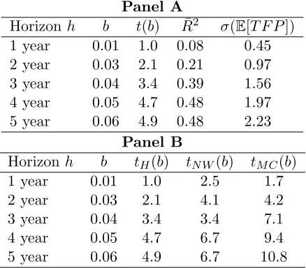
I report the results in Table 1 in two panels. Panel A documents economic significance.
A unit change in the price-dividend ratio (from 50 to 51, for example) forecasts a 0.05
percentage point increase in TFP growth over the next four years. But the real economic
significance is ascertained from the last column, which reports the expected change in TFP
for a one standard-deviation change in the IT sector’s price-dividend ratio. Focusing on
the four-year result, a one standard-deviation move in the price-dividend ratio increases
TFP growth over the next four years by two percent, or nearly a half percent per year.
To put this in perspective, real GDP growth per person is around two percent on average.
price-dividend ratio explains effectively half of the variation in TFP growth.
Panel B checks robustness by calculating the standard errors via the Newey and West (1987)
adjustment and a Monte Carlo method. Due to the persistence of the predictor variable,
es-timates of the significance of the slope coefficient can be biased (see Stambaugh (1999)). To
address this, I compute bias-adjusted small samplet-statistics, generated by bootstrapping
10,000 samples of the long horizon regression under the null of no predictability.21
Table 1: TFP-forecasting regressions I
The regression equation is T F Pt→t+h =a+b×P DtIT +t→t+h. The dependent variable T F Pt→t+h is the utilization-adjusted TFP measure provided by the San Francisco Federal
Reserve, which is a percentage change (quarterly log change times 100). The independent variable is the IT sector’s price-dividend ratio adjusted for repurchases. Data are quarterly, from 1971Q1–2012Q4. Panel A’s standard errors use the Hodrick (1992) correction equal to the forecast horizon length. σ(E[T F P]) is the standard deviation of the fitted value:
σ(ˆb×P DITt ). Panel B reports thet-statistics calculated under Hodrick (tH), Newey-West
(tN W), and a Monte Carlo bootstrap method (tM C), developed by Kilian (1999) and used
in Goyal and Welch (2008). Data sources and definitions for the IT sector are detailed in Appendix A.2.
Panel A
Horizonh b t(b) R¯2 σ(E[T F P]) 1 year 0.01 1.0 0.08 0.45 2 year 0.03 2.1 0.21 0.97 3 year 0.04 3.4 0.39 1.56 4 year 0.05 4.7 0.48 1.97 5 year 0.06 4.9 0.48 2.23
Panel B
Horizonh b tH(b) tN W(b) tM C(b)
1 year 0.01 1.0 2.5 1.7 2 year 0.03 2.1 4.1 4.2 3 year 0.04 3.4 3.4 7.1 4 year 0.05 4.7 6.7 9.4 5 year 0.06 4.9 6.7 10.8
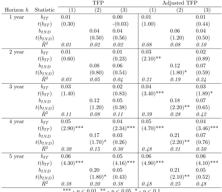
I further analyze this prediction in Table 2. Consistent with a research expenditure affecting
the economy with a lag, the effects of the price-dividend ratio are stronger at longer horizons.
21This bootstrapping procedure follows Kilian (1999) and Goyal and Welch (2008). It preserves the
Horse races are also run between the IT sector’s and the industrial sector’s price-dividend
ratios. The IT sector’s price-dividend ratio drives out the industrial sector’s when comparing
the two measures over all horizons.
These regressions capture a central fact: the price-dividend ratio of the IT sector contains
significant information about the future productivity of the economy.
1.3. Deterministic model analysis
Before proceeding to the calibrated quantitative analysis, I consider a simplified version of
the model to show that its dynamics are consistent with broad movements in the data. This
version cannot accurately match the data, so I calibrate the full model that can in Section
1.4. All insight that follows carries over to the full model.
The simplifications follow:
• The economy is non-stochastic
• The representative household is risk neutral
• Capital readjustment costs are nonexistent
• The industrial firm replaces depreciated capital, adjusting for growth
The first and second simplifications allow for a closed-form solution of the model. A
deter-ministic economy setsAt= 1 for allt. Risk neutrality sets the stochastic discount factor to
a constant Mt+1 =β = 1+1r for all t, where r can be interpreted as the real interest rate.
The third simplification sets ηk = 0. Finally, the last simplification sets It = (δ +gN∗)Kt
Table 2: TFP-forecasting regressions II
The regression equation is T F Pt→t+h =a+bIT ×P DtIT +bIN D×P DIN Dt +t→t+h. The
dependent variables are the standard TFP measure (“TFP”) and the utilization-adjusted TFP measure (“Adjusted TFP”), both of which are provided by the San Francisco Federal Reserve and are in percentage change (quarterly log change times 100). The independent variables are the repurchase-adjusted price-dividend ratios for the IT sector and the indus-trial sector. Data are quarterly, from 1971Q1–2012Q4. Standard errors use the Hodrick (1992) correction equal to the forecast horizon length. t-statistics are in parentheses. Data sources and definitions are detailed in Appendix A.2.
TFP Adjusted TFP
Horizon h Statistic (1) (2) (3) (1) (2) (3)
1 year bIT 0.01 0.00 0.01 0.01
t(bIT) (0.30) -(0.03) (1.00) (0.44)
bIN D 0.04 0.04 0.06 0.04
t(bIN D) (0.50) (0.56) (1.20) (0.50)
¯
R2 0.01 0.02 0.02 0.08 0.08 0.10
2 year bIT 0.01 0.01 0.03 0.02
t(bIT) (0.60) (0.23) (2.10)** (0.89)
bIN D 0.08 0.06 0.12 0.07
t(bIN D) (0.80) (0.54) (1.80)* (0.59)
¯
R2 0.03 0.05 0.04 0.21 0.19 0.24
3 year bIT 0.03 0.02 0.04 0.03
t(bIT) (1.40) (0.83) (3.40)*** (1.89)*
bIN D 0.12 0.05 0.18 0.07
t(bIN D) (1.20) (0.38) (2.20)** (0.65)
¯
R2 0.11 0.08 0.11 0.39 0.28 0.42
4 year bIT 0.05 0.04 0.05 0.04
t(bIT) (2.90)*** (2.34)*** (4.70)*** (3.46)***
bIN D 0.17 0.03 0.21 0.07
t(bIN D) (1.70)* (0.26) (2.20)** (0.76)
¯
R2 0.30 0.15 0.30 0.48 0.31 0.50
5 year bIT 0.06 0.05 0.06 0.06
t(bIT) (4.30)*** (4.16)*** (4.90)*** (4.10)***
bIN D 0.20 0.05 0.21 0.05
t(bIN D) (1.80)* (0.43) (2.10)** (0.52)
¯
R2 0.38 0.20 0.38 0.48 0.25 0.48
sector’s growth rate:
kt+1
Nt+1
Nt
=kt(1 +g∗N). (1.19)
Steady state
The simplifications and (1.9) imply
NtXt Kt
=
m µ
1−m1
Kt Nt
α−1
, (1.20)
and so the analysis can simply focus on the ratio kt≡ KNtt, which is an inverse mapping of
the IT-capital ratio.
From (A.2) the steady-state optimality condition for the industrial firm’s (normalized)
cap-ital choice can be rearranged to give
K N
∗
≡k∗=
α(1−m)
m µ
m
1−m
r+δ
1 1−α . (1.21)
Putting (1.20) and (1.21) together gives a simple equation for the steady-state IT-capital
ratio: N X K ∗ =
(r+δ)1−mm
αµ .
Increases in the user cost of capital (r+δ) make capital more expensive to hold and hence
increase the steady-state IT-capital ratio. As m increases, IT goods make up a larger
share of production, and thus increases the ratio. For the opposite reason, increasing the
the price paid—the user cost—for IT goods, and will thus decrease the ratio.22
Transition analysis
In this paper, I relate stock prices to the future growth rates of the economy. I structure
the analysis by starting the economy at an IT-capital ratio N0K0X0 lower than its steady-state
value N XK ∗
and then by running and observing the system’s dynamics as it converges to
its steady state:
N0X0
K0 < N X K ∗
⇔ k0 > k∗.
At this point, define the first timeT whenkt is in the ε-neighborhood of k∗ and where kt,
from time T on, will be treated as approximately equal to k∗ the following period:23
T = inf{t:|kt−k∗| ≤ε} and kt≈k∗,∀t > T.
The time T refers to how long the transition takes to get within an epsilon of the steady
state. It also introduces an element to the analysis that would otherwise be absent because
kt would asymptotically approach (and never reach in finite time)k∗. In addition, it buys
a decomposition of the ex-dividend value of an IT good at time t:
Vt−Πt≈(µ−1)
m µ
1−m1 T X s=1
βs+1kαt+s
| {z }
Transition path
+ βT+1(k
∗)α
1−β
| {z }
Steady state . (1.23) 22
Solving the present value of an IT good in the steady state gives
V∗= Π
∗
1−β =
(µ−1)X∗
1−β =
(µ−1)mµ 1 1−m
(k∗)α
1−β . (1.22)
Plugging the above equation into (1.6) gives the economy’s steady-state growth rate,
g∗N=φ+χ
1
1−ηs(βV∗)1−ηsηs −1.
23
Hence, the ex-dividend value of an IT good reflects information about the duration of the
transition path (T −t) and the distance to the steady state (|kt−k∗|).
From these simplifications, I present a proposition that summarizes the model’s salient
properties (see Appendix A.1 for details):
Proposition 2(Deterministic transition dynamics). Consider starting the economy atk0> 0 and assume there exists a sequential bound on growth, {gN,t+1}∞t=0, then
• The system xt≡ {kt, gN,t+1, Vt} converges monotonically to its steady state x∗
• The value of an IT good is an increasing function of bothT and kt for allt:
Vt(Te)−Vt(T)>0, for T > Te
∂Vt ∂kt
>0,∀t
The sequential bound on growth simplifies the proof and is consistent with the dynamics
of the full model. Its definition is in Appendix A.1. The intuition follows for the case
k0 > k∗. Because an IT good’s value is increasing in all future discounted kt’s, its initial
value is greater than its steady-state value. This incentivizes the IT sector’s research division
to develop relatively more new IT goods. Because aggregate research expenditure has
decreasing returns, kt does not immediately reach its steady state: decreasing returns act
like a variable adjustment cost, inducing a multi-period transition. As the measure of
IT goods expands tomorrow, next period’s kt decreases (and therefore next period’s NKtXtt
increases), reducing an IT good’s value. This process repeats until kt ≤ k∗+ε, at which
point the economy reaches its steady state in the following period and remains there.
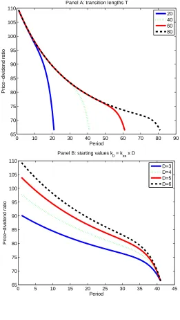
The proposition’s second bullet point implies that increasing either T or k0 increases the
value of an IT good. The difference is subtle, and clarifies the model’s use in disentangling
the two effects. Figure 1 plots the price-dividend ratio of the IT sector while varying either
the distance to the steady state (kt−k∗) or the duration of the transition to the steady
asymptotically until it nears the end of the transition, at which point the ratio starkly falls.
The bottom panel varies the distance between the initial IT-capital ratio and its steady
state. The transition is relatively more gradual for varying distances. The point to take
from this exercise is that a sharply falling price-dividend ratio signals that the end of the
transition period is near.
The transition paths of this deterministic model are qualitatively consistent with the data.
But the full model presented in the next section will also be quantitatively consistent.
1.4. Calibration and quantitative analysis
I present the model analysis in two parts. In the first part, I calibrate the model to match
historical data over the period 1974–2012. I do this in two steps:
1. Fix an initial IT-capital ratio N0X0K0 near the 1974 data point
2. Simulate an entire shock sequence{At}t=1,2,...many times for a given set of parameters
• For each simulation, compute model quantities and prices
• Average the model’s output across simulations and match it to the data
In step one, I pick the initial IT-capital ratio to also match the data’s price-dividend ratios
of both sectors. I calibrate the model in step two to agree with informative asset pricing
data: price-dividend ratios, growth rates, and discount rates. This method puts structure
on financial market data that is consistent with the underlying macroeconomic quantities.
I can then use the model’s structure to observe the remaining, and currently unobserved,
dynamics.
That said, in the second part I analyze the model’s entire transition path, which includes the
years 1974 and runs until the IT-capital ratio hits its long-run share at time T, which will
Figure 1: Deterministic model: Price-dividend ratio plots
Both panels plot the price-dividend ratio of the IT sector as a function of two of its argu-ments: the length of the transition path (T) and the distance of the model’s input ratio to its steady state (kt−k∗). The top panel varies T while the rest of the model is held
constant. The bottom panel varies Dsuch thatk0 =k∗×D while the rest of the model is held constant.
0 10 20 30 40 50 60 70 80 90
65 70 75 80 85 90 95 100 105 110
Period
Price−dividend ratio
Panel A: transition lengths T
20 40 60 80
0 5 10 15 20 25 30 35 40 45
65 70 75 80 85 90 95 100 105 110
Period
Price−dividend ratio
Panel B: starting values k
0 = kss x D
the first moment when the economy’s IT-capital ratio has crossed its unconditional expected
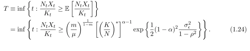
value from below:
T ≡inf
t: NtXt
Kt
≥E
NtXt Kt
= inf
(
t: NtXt
Kt ≥
m µ
1−m1
K N
∗α−1
exp
1
2(1−α) 2 σ2
1−ρ2
)
. (1.24)
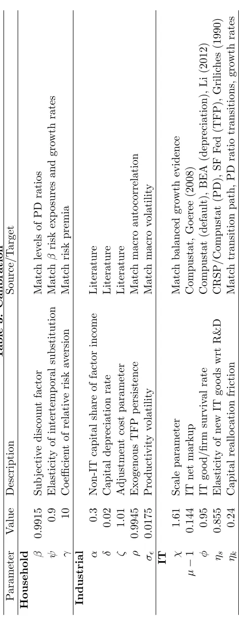
1.4.1. Calibration
Table 3 summarizes the choice of parameters. The model is calibrated at a quarterly
fre-quency. The equilibrium is computed numerically using a high-order perturbation method
(Schmitt-Grohe and Uribe (2004)) that takes into account the high volatility of stock
mar-ket prices. Note that the calibration here is unorthodox: we do not observe the entire time
series with which to estimate the parameters, because by assumption we are currently on
The calibrated parameters imply that the steady-state IT-capital ratio,E
h
NtXt
Kt
i
is 0.44, so
for every 100 units of industrial capital, there 44 units of IT capital. The model’s median
convergence time is 2033, and puts the revolution’s duration at 60 years.24
Information technology sector
The six parameters here to be calibrated areχ,φ,ηs,ηk,µ, and m. They are discussed in
turn. I set the scale parameterχ to 1.61 to match balanced growth evidence and generate
an annual consumption growth rate of two percent.
The rate of obsolescence of an IT good 1−φin the model should capture two features: a high
rate of economic obsolescence and default, as weaker firms without competitive advantages
would be expected to exit the marketplace. A BEA report by Li (2012) lists a 16.5 percent
annual depreciation rate for computers and electronics in a two-step estimation procedure
that includes an adjustment for obsolescence. This rate is higher than the 15 percent rate
applied by the BEA to generic research and development goods. In addition, I estimate the
unconditional probability of defaulting using two methods, which are described in Appendix
A.2. Both methods produce results near 3 percent. Becauseφ is interpreted as a measure,
I assume economic obsolescence and delisting are independent and add the two measures
together to get 1−φAnnual = 16.5 + 3 = 19.5 percent, or nearly φ= 0.95 at a quarterly
frequency.
To estimate ηs, I approximate (1.6) to get
log
Nt+1
Nt
≈ ηs
1−ηs
log (Et[Mt+1Vt+1]),
and then substitute this equation into (1.14) to yield
log
Zt+1
Zt
= (ρ−1) log(At) + ηs
1−ηs
log (Et[Mt+1Vt+1]) +t+1.
24
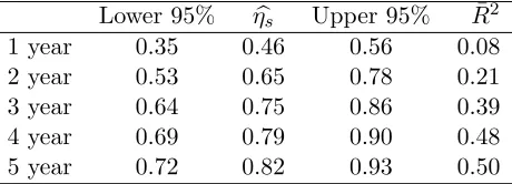
Table 4: Estimates of ηs
This table estimates the parameter ηs from the data by running the following regression: T F Pt→t+h =a+blogP DtIT +t+h. The dependent variable T F Pt→t+h is the
utilization-adjusted TFP measure provided by the San Francisco Federal Reserve, which is a per-centage change (quarterly log change times 100). The independent variable is the (log) price-dividend ratio for the IT sector, which is adjusted for repurchases. Data are quar-terly, from 1971Q1–2012Q4. The model counterpart is log (Zt+1/Zt) = (ρ−1) logAt+
ηs
1−ηs logEt[Mt+1Vt+1] +t+1. The parameter ηbs is retrieved from the estimate ofbb by the
equation: ηs(b) = 1+bb. Ninety-five percent confidence intervals are constructed using the
delta method: se(ηb) =η
0
s(bb) h
se(bb) i2
ηs0(bb), where se(bb) is computed with the Newey-West
(1987) adjustment with three lags. Data are described in Appendix A.2.
Lower 95% ηbs Upper 95% R¯2
1 year 0.35 0.46 0.56 0.08 2 year 0.53 0.65 0.78 0.21 3 year 0.64 0.75 0.86 0.39 4 year 0.69 0.79 0.90 0.48 5 year 0.72 0.82 0.93 0.50
This resembles a linear regression equation. It can be taken directly to the data to estimate
ηs. I provide estimates in Table 4. Because the price-dividend ratio better explains TFP
variation at a longer horizon, estimates of the four- and five-year horizon are considered.
Estimates at these horizons range from 0.69 to 0.93. Griliches (1990) also provides some
estimates, which range from 0.6 to 1.0, depending on the use of cross-sectional or panel
data. I pick 0.855.
Estimating the parameter that governs the cost of capital readjustment ηk is difficult.
Jo-vanovic and Rousseau (2002) provide estimates of learning laws, a friction of capital
real-location, for general purpose technologies, like IT, within a range of 0.2 to 0.62. I choose
0.24. I discipline this choice by having this single parameter match the S-shaped diffusion
dynamic of the IT-capital ratio, the transitions of both sectors’ price-dividend ratios, and
the IT sector’s net entry and sales growth rates.
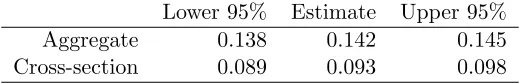
Table 5: IT sector markups
This table reports average markups of IT firms over the annual period 1974–2012. Markups are estimated byµ= 1−1x −1, wherex is the EBITDA-sales ratio, defined below. The row “Aggregate” refers to the sum of EBITDA divided by the sum of sales, and then temporally estimates the average value. The row “Cross section” takes the cross-sectional median of all firms in every year, and then temporally estimates the average value. Standard errors have the Newey-West (1987) adjustment with three lags. Data are defined in Appendix A.2.
Lower 95% Estimate Upper 95% Aggregate 0.138 0.142 0.145 Cross-section 0.089 0.093 0.098
measure accurately, especially given the IT sector’s heterogeneity of products.25 One study
by Goeree (2008) finds that the median markups on personal computers across the total
industry range from 5 to 15 percent, depending on the degree of information possessed
by consumers in her limited-information model of consumer behavior. Moreover, direct
estimates (see Table 5) based on the IT sector’s average EBITDA-to-Sales ratio, a measure
of markups, are 9.5 and 14 percent, depending if cross-sectional medians or aggregate means
are used. I use 14.3 percent.
The IT share of factor income parametermdetermines the importance of IT in the
produc-tion. This is unknown by construction, because the steady state has not yet been observed.
The choice is disciplined, however, by the balanced growth condition in (1.11) which specifies
m given µand α, two parameters that are plausibly easier to measure.
Industrial sector
The parameters here areα,δ,ζ,ρ, andσ. The ranges of these parameters have largely been
agreed upon by the literature. A usual value for α is in the neighborhood of a third, and
I use a value of 0.3. I set the quarterly rate of depreciation δ to 0.02, or around 8 percent
at an annual rate. The adjustment cost parameter ζ is set to 1.01, which falls in line
25For example, software and hardware manufacturers abide by different standards. Hardware
with estimation evidence (see, for instance, Jermann (1998), Kaltenbrunner and Lochstoer
(2010), and Croce (2012)). I choose the persistence parameter ρ to be an annualized value
of 0.978 to match the first-order autocorrelation of consumption growth. Remember that
measured productivity is a composition of the exogenous and endogenous components in
the model. Finally, I pick the volatility of the exogenous TFP process σ to be 0.0175 to
generate plausible macroeconomic volatilities.
Households
Households are characterized by recursive preferences, which are governed by three
parame-tersγ,ψandβ. Substantial empirical work has been done on these parameters, see Bansal,
Kiku and Yaron (2012), and this is followed here by settingγ = 10,ψ= 0.9, andβ= 0.9915
to produce reasonable levels for price-dividend ratios. The elasticity of substitution
parame-ter is usually assumed to be greaparame-ter than one in much of the long-run risks liparame-terature (Croce
(2012), Bansal and Yaron (2004)). The model, however, requires a value less than one to
match the observed relationship of risk exposures (betas), as described in the next section.
1.4.2. Transition calibration
I match five transition paths: the IT-capital ratio, both sectors’ price-dividend ratios, and
the IT sector’s average sales and net entry growth rates. The first path is the variable of
interest. The latter four ensure that the model’s asset pricing variables are consistent with
financial market data. I discuss discount rates in the next section.
IT-capital ratio
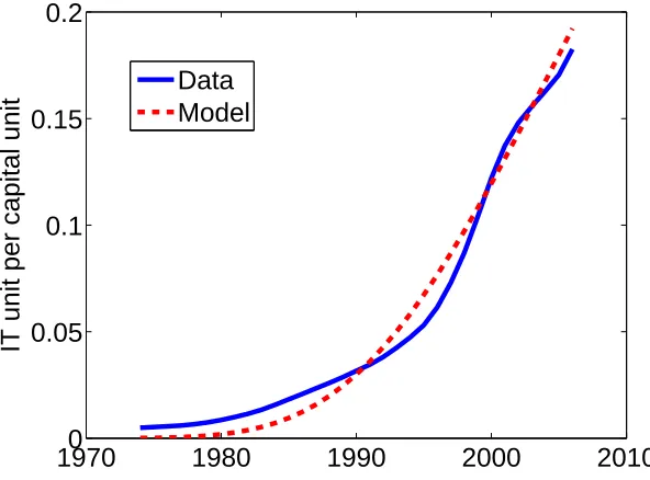
Figure 2 plots the IT-capital ratio of the data versus that generated by the model. I calibrate
the model to match the initial IT-capital ratio to as close to the 1974 data point as possible,
but I also require the model to be consistent with the data on price-dividend ratios as well.
Figure 2: Model calibration I: Input ratio
This figure plots the IT-capital ratio, the ratio of the IT sector’s quantity of capital services to the industrial sector’s. Capital services are direct estimates of factor income which are based on flows derived from constructed constant-quality capital stock indices. The IT sector is defined as the sum of software, hardware, and communications as listed in the Bureau of Economic Analysis; the industrial sector comprises the remaining 62 asset classes. See Jorgenson and Stiroh (2000) for details. A detailed description of the origin of this figure is in Appendix A.2. I fix an initial IT-capital ratio N0X0K0 <EN XK and calibrate the model to match the length and curve of the data.
1970
0
1980
1990
2000
2010
0.05
0.1
0.15
0.2
IT unit per capital unit
Data
Model
its construction. An important disciplining device is the model’s other transitions.
Price-dividend ratios
The price-dividend ratio of the IT sector is defined in (1.18). The price-dividend ratio of
the industrial sector is qtKt+1/Dt. Table 6 lists the values of the start- and end-points of
the model that is consistent with the data available for the IT-capital ratio. In Figure 3
I plot the system’s transitions. The model is able to match the industrial sector’s
price-dividend ratio to the time series data. Within its confidence bounds, the model can capture
the run-up in prices during the dot-com boom and even the drop during Great Recession
of 2008. The IT sector’s price-dividend ratio of the model is able to capture the trend of
ratio is consistent with that observed as well. The model has difficulty in generating the
magnitude of the dot-com boom. Although this is not surprising because the model is not
calibrated to match an episode of a “bubble”. What is important is that the data reverted
back to the model’s implied value after the boom.
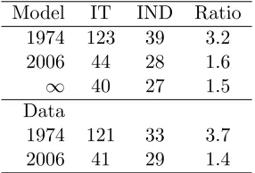
Table 6: Price-dividend ratios
This table reports price-dividend statistics generated by the model and compares them to the data. The model takes its calendar-time counterparts and estimates the average (across simulations) value of the price-dividend ratios of the IT and industrial sector. The data comes from an average of the previous sixteen quarters from data at year-end 1974 and 2006. The value∞ represents the model’s steady-state value. I discuss the construction of price-dividend ratios in Appendix A.2.
Model IT IND Ratio 1974 123 39 3.2 2006 44 28 1.6
∞ 40 27 1.5
Data
1974 121 33 3.7 2006 41 29 1.4
IT sector average sales growth rates
I plot the transition of the IT sector’s average sales growth rate in Figure 4. The model
matches the fast, initial increase displayed by the data and then its drawn out path to
convergence. This fast increase is consistent with a competition driving down the sales
generated per firm. In the model, initially few firms dominate the marketplace. Over time,
as more firms enter the marketplace, the industrial firm reduces the quantity demanded of
each IT firm’s good. Consequently, sales and profit earned per firm falls.
IT sector net entry rates
I depict in Figure 5 the transition of the IT sector’s net entry rate. The model matches the
sharp decline displayed initially by the data and then its drawn out path to convergence.
The model is unable to get its mean to be negative to match the data after the dot-com
Figure 3: Model calibration II: Price-dividend ratios
This figure plots time series paths of the sectors’ price-dividend ratios. The dashed line is the model’s average simulation path. The dotted lines are two times the model’s standard errors. Standard errors are estimated from the standard deviation of point estimates across simulations. Ten-thousand simulations are run. The solid line is data. The top figure is the IT sector; the bottom is the industrial sector. In the data, I calculate repurchase-adjusted price-dividend ratios, as described in Appendix A.2. Data are quarterly and are smoothed with a Hodrick-Prescott filter with a smoothing parameter equal to 1600.
1980 1990 2000 2010 0
50 100 150
IT sector PD ratio
Data Model 2*SE
1980 1990 2000 2010 0
10 20 30 40 50 60
Industrial sector PD ratio
Figure 4: Model calibration III: IT sector’s average sales growth rate
This figure plots the average sales growth rate per firm of the IT sector. The dashed line is the model’s average simulation path. The dotted lines are two times the model’s standard errors. Standard errors are estimated from the standard deviation of point estimates across simulations. Ten-thousand simulations are run. The solid line is data. The data use Compustat data for the IT sector to calculate aggregate sales growth rates per public IT
firm (Nt): log
y
t+1 yt
, where yt =
PNt i Salesi,t
Nt . Data are quarterly and are smoothed with a Hodrick-Prescott filter with a smoothing parameter equal to 1600. In the model, the variable is logΠt+1
Πt
. IT firms are identified by NAICS codes in Appendix A.2.
1980 1990 2000 2010 −50
−40 −30 −20 −10 0 10 20
Average sales growth rate (%)