Marine sediment classification using the chirp sonar

University of New Hampshire

University of New Hampshire Scholars' Repository

Affiliate Scholarship

Center for Coastal and Ocean Mapping

1-1992

Marine sediment classification using the chirp

sonar

Lester R. LeBlanc

Larry A. Mayer

University of New Hampshire, [email protected]

Manuel Rufino

Steven G. Schock

John King

University of Rhode Island

Follow this and additional works at:

https://scholars.unh.edu/ccom_affil

Part of the

Geology Commons

,

Oceanography and Atmospheric Sciences and Meteorology

Commons

, and the

Sedimentology Commons

This Article is brought to you for free and open access by the Center for Coastal and Ocean Mapping at University of New Hampshire Scholars' Repository. It has been accepted for inclusion in Affiliate Scholarship by an authorized administrator of University of New Hampshire Scholars' Repository. For more information, please [email protected].

Recommended Citation

Marine sediment classification using the chirp sonar

Lester R. LeBlanc

Department of Ocean Engineering, Florida Atlantic University, Boca Raton, Florida 33431-099!

Larry

May,er

Dalhousie University, Halifax, Nova Scotia B3H 4J1, Canada

Manuel Rufino

Department of Ocean Engineering, University of Rhode Island, Narragansett, Rhode Island 02882

Steven G. Schock

Department of Ocean Engineering, Florida Atlantic University, Boca Raton, Florida 33431-0991

John King

Graduate School of Oceanography, University of Rhode Island, Narragansett, Rhode Island 02882

(Received 1 March 1991; accepted for publication 12 September 1991 )

The chirp

sonar

is a calibrated

wideband

digital

FM sonar

that provides

quantitative,

high-

resolution, low-noise subbottom data. In addition, it generates an acoustic pulse with special

frequency

domain

weighting

that provides

nearly

constant

resolution

with depth.

The chirp

sonar

was

developed

with the objective

of remote

acoustic

classification

of seafloor

sediments.

In addition

to producing

high-resolution

images,

the calibrated

digitally

recorded

data are

processed

to estimate

surficial

reflection

coefficients

as well as a complete

sediment

acoustic

impulse

profile.

In this

paper,

surficial

sediments

in Narragansett

Bay,

RI are used

to provide

ground

truth for an acoustic

model.

Quantitative

acoustic

returns

from the chirp

sonar

are

used to estimate surficial acoustic impedance and to predict sediment properties. A robust

acoustic sediment classification model that uses core samples to account for the local

depositional

environment

has

been

developed.

The model

uses

an estimate

of acoustic

impedance

to predict

surficial

density,

porosity,

compressibility,

and rigidity.

The comparisons

show

a high correlation

between

the core-determined

sediment

properties

and the estimates

obtained from acoustic measurements.

,

PACS numbers: 43.30.Ma, 43.30.Vh

INTRODUCTION

The remote classification of marine sediments by acous- tic means requires a quantitative, high-resolution profiling system as well as a solid theoretical and/or empirically de- rived basis upon which to convert the acoustic measure- ments into the desired sediment properties. Recent advances in subbottom profiler design have produced high-quality

data suitable for sediment classification work. 1 The collec-

tion and acoustic analysis of cores taken in conjunction with these seismic surveys provides a database for developing al- gorithms for sediment property prediction as well as "ground truthing" of the profiler's ability to remotely identi- fy sediment type.

In this paper we describe an experiment conducted in Narragansett Bay, RI, using the chirp sonar, a calibrated, wideband (2-10 kHz), digital FM sonar that provides quan- titative, high-resolution ( • 10 cm), deep penetration

( • 100 m) subbottom

data.

1'2 The chirp sonar

was devel-

oped with ONR funding to support the objective of remote

acoustic classification of marine sediments. In addition to

producing high-resolution images of the subsurface, the cali- brated digitally recorded data can be processed to provide surficial reflectivity estimates. Subbottom returns can also

be processed for attenuation I and when corrected for at-

tenuation, chirp sonar profiles can provide a reflectivity se- ries well suited for acoustic impedance inversion.

Along with chirp sonar profiles, cores were collected in Narragansett Bay. These cores were analyzed for velocity, density, porosity, grain density, and grain size. There is a wealth of literature describing empirical studies of sediment

physical and acoustic property relationships. 3-8 These stud-

ies have resulted in a number of regression equations that can often be successful in their ability to predict one property from another (typically within a given depositional environ- ment) but have provided only limited insight into the inter-

action between acoustic waves and marine sediments. Theo-

retical studies of sediment-acoustic wave interaction, on the

other hand, particularly those of Biot 9'1ø and Stoll ll have

used sophisticated formulations that take into account the sediment frame properties. In this paper we have initially taken a simplified view of the manner in which a normally incident acoustic wave emitted from an acoustic profiler in- teracts with a fully saturated marine sediment. In our model, we have assumed that the marine sediment is macroscopical- ly homogeneous and that most of the acoustic-marine sedi- ment interaction can be accounted for by the bulk properties of the sediment, i.e., porosity, specific gravity, elasticity, and

rigidity. The problem of extracting quantitative sediment

parameters from normal incidence reflection profiles poses a

difficult challenge. Even under the most ideal conditions, the

acoustic wave energy is scattered by the random unevenness of the seafloor and the inhomogeneities within the sediment. In order to extract any meaningful information from the stochastic acoustic signal that is returned from the seabed, a model with significant averaging of the estimated param- eters is required. The model developed in this paper has

enough flexibility to model most surficial sediment deposi-

tional environments. Further, the model can be calibrated to

a local area by using average grain density, grain elasticity, and a rigidity constant obtained from core samples. In this

manner, chirp profiler data obtained using a 2-to 10-kHz

swept FM is processed to provide reasonable predictions of

sediment type.

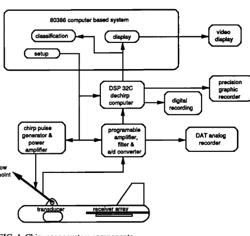
I. CHIRP SONAR DESCRIPTION

The chirp sonar system shown in Fig. 1 uses a linearly

swept FM pulse that typically covers the range of frequen-

cies from 2-10 kHz. The rectangular acoustic projector is constructed from four wideband piston type transducers and the acoustic receiver is a ceramic line array. The acoustic arrays are mounted in a tow vehicle that is designed for pro- filing at ship speeds varying from 0 (drifting) to 10 kn. Sepa- rate receiving and transmitting arrays are used to preserve linearity and to allow simultaneous transmission and recep- tion. The receiver array signal is digitized with a 16-bit A/D converter at a sampling rate of 30 kHz. To achieve the theo-

retical temporal resolution predicted by the inverse of the

bandwidth, the chirp pulse is compressed using a matched filter that correlates the chirp return signal with a replica of

the outgoing pulse. The correlation process is implemented

with a discrete Fourier transform which is calculated in real

time with a pipeline array processor. The hardware used to

accomplish this is a AT&T DSP 32c processor controlled by

80386 computer based system classification

DSP 32C

dechirp

precision graphic

tow

point

chirp pulse programable

generator & amplifier,

power filter & a/d converter

DAT analog

recorder

a 80386 microcomputer. The compressed pulse resulting from this signal processing procedure has a time duration approximately equal to the inverse of the bandwidth of the chirp pulse. Good resolution is an important factor in sedi- ment classification because it provides a more precise picture of the true geologic variability (the impulse response of the sediment), and thus permits accurate determination of the depositional processes. When the time duration of the pro- cessed pulse is too large, individual reflections will be

lumped together with random phase, thus making it difficult

to estimate impedance and to examine geologic processes. In addition to the pulse compression correlation pro- cessing achieves a signal processing gain over the back- ground noise. This gain is approximately ten times the log of the time-bandwidth product. To equal the performance of the chirp sonar pulses that were used in this experiment, a conventional pulse sonar would have to operate at a peak pulse power of 100 times larger than the chirp pulse.

Another important feature that enhances the ability of the chirp sonar system to classify sediments is realized by the deconvolution of the system response from the output pulse. The sonar system impulse response is measured in the labo- ratory and is used to design a unique output pulse that will

prevent the source from ringing. In addition to this, the chirp

wavelet is weighted in the frequency domain so as to have a Gaussian-like shape. As the Gaussian-shaped spectrum is attenuated by the sediment, energy is lost but its bandwidth

is nearly preserved. •2 Thus even after being attenuated by 20

m of sand, the chirp pulse has approximately the same reso- lution as an unattenuated pulse. This feature simplifies the mathematics of inverting the time series to obtain the imped- ance profile of the sediment. In addition to a loss of total energy, attenuation causes the center frequency of the chirp pulse spectrum to shift to a lower frequency, thus allowing us

to estimate the attenuation of the sediment.

Another important feature of the chirp sonar is the re-

duction of side lobes in the effective transducer aperture.

The wide bandwidth of the FM sweep has the effect of smearing the side lobes of the transducer and thus achieving a beam pattern with virtually no side lobes. The effective

spatial beamwidth obtained after processing the chirp signal

is 20 ø measured to the - 3-dB points. This feature is appar- ent when inspecting the sample profile record shown

in Fig. 2.

Since the transmitted chirp pulse is highly repeatable and its peak amplitude is precisely known, the sediment re- flectivity values can be estimated from the peak pulse ampli- tude measurements of the bottom returns. In this experi- ment, peak pulse amplitude was recorded while surveying a section of Narragansett Bay. When an interesting feature

appeared, grab samples were taken at that station. The sam-

ples were analyzed for grain size, porosity, and sound speed, and then compared to the chirp sonar estimated sediment impedance.

FIG. 1. Chirp sonar system components.

II. BOTTOM LOSS MEASUREMENT AND SEAFLOOR

CLASSIFICATION

When an acoustic wave traveling through the water en- counters the sediment boundary of the seafloor, reflected

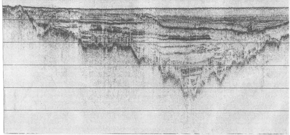
FIG. 2. Typical chirp profile in Narragansett Bay, RI taken between the Wickford breakwall and Hope Island; horizontal extent is about 1500 m and vertical

scale is 10 m between grid lines. The record reveals: a glacially excavated river valley overlain by approximately 30 m of varved glacial lake deposits; a fluvial

uncomformity at the top of the lake sediments and; approximately 10 m of marine estuarine sediments deposited with the most recent rise of sea level.

and transmitted waves are generated at the fluid-sediment

boundary. For a simple harmonic plane wave normally inci- dent on a plane boundary, the Rayleigh reflection coefficient

is given by,

R = (p•,c•, --pwCw)/(p•,c•, +pwCw) (1) and the bottom loss (BL) of the plane wave at normal inci- dence is then given by

BL = -- 20 Log]o (R). (2)

Initially, we are using this equation as the basis for classify- ing surficial sediments on the seafloor.

Obviously, there are many approximations that can modify our analysis; seafloor roughness, planar wave as-

sumption, other waves generated at the boundary, •3 and

bottom curvature to mention a few. To some extent, the ef-

fects of seafloor roughness can be reduced by averaging the

reflected values. In addition to the mean value, the reflected

pulse width and pulse amplitude variance are indicators of sediment types. In this experiment, we used the mean ampli- tude to determine bottom type. In several instances, gaseous sediments were brought up in the grab corer and in each case, a broadening of the reflected pulse was noticed. In shal- low coastal areas, gaseous surficial sediments are quite often present. These sediments present a large reflection coeffi- cient while providing volume scattering that lengthens the

pulse returned from the boundary. TM In the future, our pro-

gram will include these effects as well as accomplish a math- ematical impedance inversion to obtain the acoustic impulse response of the sonified column of marine sediment.

109 J. Acoust. Soc. Am., Vol. 91, No. 1, January 1992

/

III. RELATIONSHIP BETWEEN SEDIMENT PROPERTIES

AND BOTTOM LOSS

An'unconsolidated marine sediment is a porous and

loose structure whose interstices are filled with seawater.

Therefore, it can be thought of as composed of a fraction

which is seawater and a remainder which is solid material.

Porosity, which is defined as the ratio of the volume of voids

between the grains of a sediment to the total volume of the sediment aggregate is therefore an important parameter in describing the way marine sediments react acoustically.

The relationship between bulk density of a marine sedi- ment and porosity is given by

Pt, =Pw n +pg(1 -- n), (3)

wherep& is the bulk density of the sediment, Pw is the density

of bottom water, log is the density of the solid material (grain

density), and n is the porosity of the sediment. This is a simple linear relationship that is easily derived by consider- ing the total mass of material enclosed in a unit volume made up of two materials. In Eq. (3), the porosity n is easily ob-

tained as a function of density:

11--

(pg

--Pw)/(Pg

--Po

).

(4)

The compressional wave velocity for a wave in isotropic elas-

tic media

• is well known

and is given

by

( 1//3t,

-I-

4/-t/3)

c• = , , (5)

Po

where/% is the bulk compressibility of the water saturated

sediment, and p is the bulk modulus of rigidity. For small

pressure

perturbations,

the bulk compressibility

is linearly

dependent on the porosity of the sediment.

For an adiabatic process, the compressibility is defined

as the fractional change in a unit volume of material for a

given change in pressure:

= a_[.

(6)

Thus the fractional change in a unit volume of water satu-

rated sediment is a linear combination of the individual com-

pressibility of each material, and is given by

=/3wn +/3g (1 - n),

(7)

where/3w

is the compressibility

of water

and/3g

is the com-

pressibility

of the solid material (grain compressibility).

The characteristic acoustic impedance (P0 co ) of the marine

sediment is now obtained by combining Eqs. (3), (5), and

(7) as follows,

Z0 --poco

= Z•(•

+pR(1--n)

+ •- /flJ•

4

[ n + p• (1- n

) ] ,

) 1/2

(8)

where

PR :•Og/•Ow

is the grain density

relative

to bottom

water,

•2-3; p• is the

density

of bottom

water,

1025

kg/m3;

/JR =/3g/13•

is the grain

compressibility

relative

to bottom

water, •0- 1;/3• is the compressibility of bottom water,

42.94

X 10- 11

m2/N (Ref.

7); and Zw = (p•//3•) 1/2

is the

impedance

of bottom

water, 1.549

X 106 kg/m2s (note--

p•,pg,/J•,lJg,

referred

to 1 atm and 23 øC).

The compressional wave velocity of the sediment is ob-

tained in the same manner by c. ombining Eqs. (3) and (7)

with (5):

the averagepR,/5'R, and p corresponding to the coastal depo-

sitional environment that the samples were taken from. The curve fitting process is carried out in two stages: The first stage is initiated by starting with an initial estimate of rela- tive density, relative compressibility, and rigidity. The first two of these starting values are varied until a minimum least- squares fit is obtained between the measured impedance val- ues and the impedance values predicted by Eq. (8). In the second stage, the second group of measurements (imped- ance density) are used to find the rigidity constantthat again produces a least-squares fit of Eq. (8) to the actual imped- ance measurements. In order to accomplish this, the density values were first converted to porosity by using Eq. (4) and then porosity data was used directly in Eq. (8) to calculate impedance. The process of adjusting the PR and/3R in the first least-squares solution and then rigidity p in the second solution, is repeated in this same manner until the errors in both curves are globally minimized. This procedure is used to obtain a set of constants PR,/JR, and p that provides us with a calibration of Eq. (8) to a given depositional environ-

ment.

Before carrying out the above-mentioned procedure to solve for the sediment parameters, another minor refine-

ment was required to the rigidity term in Eq. (8). Based on a

careful observation of the data collected for this study, it is

suggested that rigidity of surficial sediments is dependent on

the percentage of solid content in a marine sediment. This

concept was empirically tested by assuming the following

equation for the dependence of rigidity on density,

P = Po (Po/P,, -- 1 )•, (10)

where Po is the rigidity constant--a function of depositional

environment,

(Po/P,, -- 1 ) is a quantity

that is proportional

to the solid material in a unit volume of marine sediment,

and

r/is an arbitrary

exponential

power

constant

(r/= 1 ).

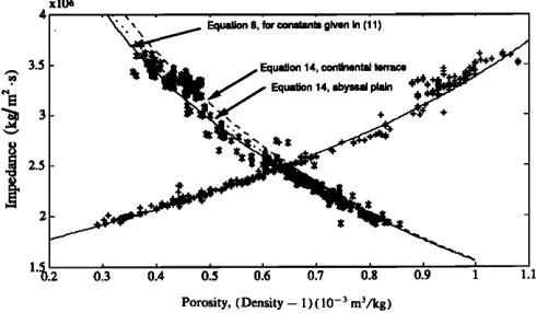
Figure 3 is a plot showing the impedance versus porosity

and impedance versus (density- 1); both "actual data"

1 •

Cb m Cw

[n

(1 -n)] [n

4/3p/3•

)•/2,

(9)

+ [n

+PR

(1

-- n)]

and the least-squares fit of Eq. (8) to the data are plotted.

The rms error in the curve fit is about 4% indicating a high

correlation between the group of data taken from Refs. 3-7

and the theory developed herein. Prior to including the rigid-

where

c• = x/1//•op•,

is the

compressional

wave

velocity

of

bottom water, 1.504 X 103 m/s.

Equations

(8) and (9) relate

the porosity

and

rigidity

properties of a given marine sediment sample to acoustic

impedance

and

sound

velocity.

In a given

depositional

envi-

ronment,

it is hypothesized

that the relative

grain

densitypR

and

the

relative

grain

compressibility/JR

in

Eqs.

( 8

) and

(9)

are

nearly

constant

and

therefore

porosity

and

rigidity

are

the governing factors in determining the acoustic impedance of the surficial sediments.

In order to test this hypothesis, independent sets of im- pedance versus density, and impedance versus porosity data

37

were collected from five references. - All of the samples were near-surface samples taken in coastal regions (terrigen-

ous sediments). The data from these references were used in

a nonlinear least-squares curve fitting process so as to obtain

xlO•

Equation 8, for constants given in (11)

Equation 14, continents] terrace Equation 14, abyssai plain

+

0.3 0.4 0.5 0.6 0.7 0.8 0.9 1 1.1

Porosity, (Density -- 1 ) ( 10 -3 m3/kg)

FIG. 3. Impedance as a function of both porosity (.) and (density- 1 )

( + ) for actual data taken from five references and the least-squares curve

fitting of Eq. (8) to the data. Other curves are from Ref. 6.

ity term in Eqs. (8) and (9), the rms error was about 5%

greater.

In carrying out the least-squares fit, the power r/in œq. (10) was allowed to vary so as to determine its relationship to various depositional environments. In all cases, it was found that r/was very close to 1, and based on this result, r/ was fixed at a value of one and Po was recalculated for all of the data sets. It is not too unreasonable to expect the rigidity of a sediment to vary in a linear manner (r/= 1 ) with the composition of solid material in the marine sediment. The remainder of the constants obtained by the least-squares fit- ting procedure are in the proper range for terrigenous sedi- ments and are given here:

grain

density

Pg =PwPR

= 2670 kg/m

3,

grain

compressibility

fig =/3w/3R

= 4.85

X 10- • m2/N,

rigidity constant Po = 0.0005 X 10 TM N/m 2. ( 11 )

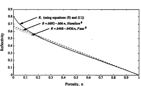
The plane-wave pressure reflection coefficient is easily related to the porosity or density by noting from Eq. ( 1 ),

R = (Z•, -- Z,,, )/(Z•, + Z,,, ), (12)

where Z is obtained either by direct substitution of the poros- ity, n into Eq. (8) or indirectly, by finding the porosity from the density values using Eq. (4), and then substituting into Eq. (8). The solid line in Fig. 4 is a plot of reflection coeffi- cient as a function of porosity. It is the result of using the

previously

derived

grain characteristics

(pg,t3g,po)

in Eq.

(8). Faas

s used

density

and compressional

sound

velocity

data from four separate references to compile impedance data. The data were then used in a linear least-squares fit to obtain an empirical equation that relates the reflection coef- ficient to porosity,

R =0.6468--0.6456n (0.35<n<0.85). (13)

Data taken from this equation are plotted for comparative purposes on the same figure. The empirical equation is only valid in the limited range given above. However, in this range, there is an excellent correspondence between our Eq. (8) derived from basic physical principles, and the empirical relationship given by Eq. (13). Part of the high degree of correspondence is attributed to some overlap in data sets used in both methods. Nevertheless, the comparison is en-

0.9 0.8 0.7 0.6

0.5 0.4

0.3 0.2 0.1 0 0

•X,•

R,

(using

equations

(8)

and

(11))

' '•'

:"

'•,'•

.-,.•.

'•'

,

,

011 012 013 014 015 016 0.7 0.8 0.9 Porosity, n

FIG. 4. Hamilton's and Faas's empirical equations for reflection coefficient compared to Eq. (8) derived in text.

couraging and points to a more quantitative way of charac- terizing the depositional environment. To account for differ- ent depositional environments, Hamilton proposed three empirical equations for relating porosity to reflection coeffi-

cient:

R = 0.6692 -- 0.666n; continental terrace,

R = 0.6199 -- 0.607n; abyssal hill,

R = 0.6461 -- 0.646n; abyssal plain, (14)

where 0.35<n<0.85.

For comparison, data from Hamilton's continental ter- race equation are also plotted in Fig. 4. All of these empirical equations constitute attempts to relate the functional behav- ior between reflection coefficient and porosity to a given de- positional environment in a qualitative manner. Using the

method

developed

in this paper,

we are able to establish

a

quantitative method of characterizing the depositional envi- ronment. This is accomplished by specifying grain density, compressibility, and rigidity values in Eq. (8). In order to obtain these parameters, in a given geographic area, a limited set of cores and knowledge of the geological depositional processes involved could be combined to provide an estimate of the constants. Using this simple calibration procedure, normal incident reflectivity values obtained from the chirp sonar are used to predict porosity, density, grain size, rigid-

ity, and sound velocity.

Hamilton 6 developed another empirical relationship

that can be used to provide an estimate of grain diameter from porosity:

n = 31.05 + 5.52•, (15)

where ß = -log2 (mean grain diameter in mm), and

1<•<9.

The correlation between porosity and mean grain diam- eter is not as well defined as the correlation between porosity and density. The standardized error is of the order of 30%. Theoretically, the actual size of each grain in a sediment has no influence on the porosity if the grains were uniform

spheres. In actuality, as the grain size decreases, friction,

adhesion, and bridging increases. Thus a correlation exists between mean grain diameter and porosity but the relation- ship is complex.

For the purpose of providing a general class name to a given sediment in this experiment, Hamilton's table for the

continental terrace (Table I) was used to relate measured

TABLE I. Sediment reflection coefficient and bottom loss for continental

terrace. 6

Sediment type Average reflection coefficient

Coarse sand 0.4098 ( -- 7.8 dB) Fine sand 0.3749 ( -- 8.5 dB)

Very fine sand 0.3517 ( -- 9.1 dB)

Silty sand 0.3228 ( -- 9.8 dB)

Sandy silt 0.2136 ( - 13.4 dB)

Sand-silt-clay 0.2504 ( -- 12 dB)

Clayey silt 0.1767 ( -- 15 dB)

Siltyclay 0.1586 (--16 dB)

reflection coefficient values to sediment type.

This general relationship between class names and sedi-

ments is based on a recommendation by Shepard •6 which

accounts for proportions of sand, silt, and clay present. A general relationship like this is possible since sands have less porosity than silts and clays and the latter are more porous.

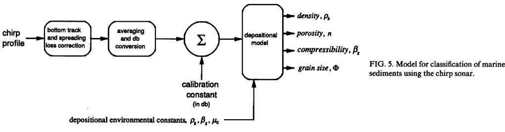
IV. CLASSIFICATION OF MARINE SEDIMENTS USING

THE CHIRP SONAR

Since the chirp sonar is a digital FM system, the ampli-

tude of the correlated sediment-water interface reflection is

accurately measured and recorded. As shown in Fig. 5, the

reflection coefficient of the first bottom arrival is detected

and corrected for geometric spreading. These raw values are averaged over several returns ( • 10-100) to reduce the un- desirable effects of noise, scattering, and an uneven bottom.

The unscaled reflection coefficient values are then converted

to dB values, Rdb = --20 log(R). Using the sonar equa- tion, the system calibration constant is now subtracted from

the estimated, unscaled reflection values to obtain the reflec-

tion loss of the seafloor. The system calibration constant used in this equation can be obtained by either a direct tank calibration, or by an indirect method using a known seafloor type, or a flat reflecting plate target placed at a fixed distance from the transmitter and receiver pair. The impedance esti-

mate of the seafloor is now obtained from

z• =Z•[(I +R)/(] -R)]. (16)

Equations ( 8 ) and (9) are now solved to obtain porosity and sound velocity estimates for the marine sediment. Equation (3) is used to find a density estimate, Eq. (10) to find a rigidity estimate and finally, Eq. (15) is used to obtain an estimate of average grain size.

V. EXPERIMENT AND RESULTS

A seafloor reflectivity survey was carried out in Narra- gansett Bay, RI in May 1990 and a second experiment later in Sept. 1990. The chirp sonar (Fig. 1 ) system was set up and calibrated to transmit a 20-ms pulse ranging in frequency from 2 to 9 kHz at a rate of twice per second. In the first experiment in May, the system was calibrated by using a large area of seafloor of known sediment type (sand, sandy silt, clayey silt) in Narragansett Bay. Other areas in the bay were then analyzed by the chirp system and compared to

previous ground truth (cores) data. In the second experi- ment, sonar data and grab sample cores were taken at nine selected sites in the same proximity of the May survey. The cores were analyzed for sound velocity, density, and porosity and used to calibrate our depositional environment equa-

tions.

The geographic area in which these experiments were conducted is the West passage of Narragansett Bay, RI. Narragansett Bay, like many estuaries in the northeast is a

glacially deepened river valley that was excavated during the

last glaciation (approx. 18 000 years before present). As the glacier retreated, glacial till was deposited over bedrock, a

glacial lake formed behind a dam of glacial debris and ap-

proximately 30 m of varved, lake sediments were deposited

over a period of several thousand years (a typical profile is

shown in Fig. 2). With the breaching of the glacial dam and

the rise of sea level, several erosional unconformities formed

on the surface of the lake sediments followed by the depo- sition of approximately 10 m of fine-grained marine estuar-

ine sediments (Fig. 2; Peck and McMaster •7 ).

The surficial sediments of Narragansett Bay have been

studied

by McMaster;

•8 the distribution

of sediment

types

in

the West Passage is shown in Fig. 6. In this region, McMas- ter identified five surficial sediment types based on the rela- tive percentages of material defined as gravel (> 2 mm); sand (2-0.062 mm); silt (0.062-0.005 mm); and clay

( < 0.005 mm). The distribution of these sediments is a func-

tion of the interactions among: river supply, erosion of pre- existing deposits, redistribution by tidal and nontidal circu- lation patterns, and anthropomorphic effects (dredging).

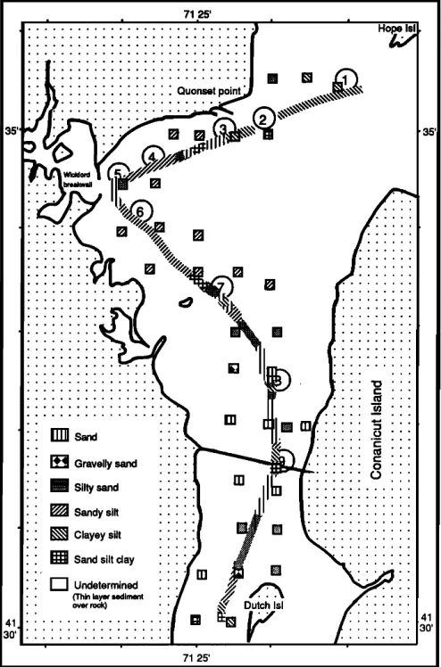
During the May 1990 survey, a south-north line be-

tween Dutch Island and the Wickford breakwater wall and a

west-east line between the Wickford breakwater and Hope Island were run with the chirp sonar (Fig. 6). Loran C navi- gation, with three calibration points along the ship's track, provided accurate ( q- 10 m in the absence of abrupt atmo- spheric changes) positional information. Figure 2 shows a sample chirp sonar profile taken near the Wickford Harbor entrance. This profile, fairly typical of those from Narragan- sett Bay, shows the succession of geologic features described

above.

The large areas of sand north of the Jamestown Bridge, the sandy-silt area west of Wickford Harbor, and clayey silt around Hope Island provided excellent data for calibration of the chirp sonar. In each of these areas, 360 reflection val-

ß bottom track averaging porosity, n

chirp

odel

profile

- I•s

correctior•J

- Lconversion

compressibility,

fi

grain size,

calibration constant

(in db)

alepositional environmental constams, p•,,Ss, •

FIG. 5. Model for classification of marine

sediments using the chirp sonar.

71 25'

...

:::::::::::::::::::::::::

FITI! Sand ' ' '

B• Gravelly sand .1• si,y s=d • Sandy silt I• Clayey silt I• Sand silt clay

I•1 Undeterrnined

(Thin layer sediment over rock)

...

...

...

ß

71 25'

rn

FIG. 6. Comparison of chirp sonar predicted sediment characteristics along the ship's track with core sites taken from McMaster (Ref. 18). Circles

mark Sept. 1990 core sites.

ues were acquired and averaged. This corresponds to about 500 m of the ship's track in each area. The average and stan- dard deviation of the sonar's output (corrected for spherical spreading) are given in Table II for each of the three calibra-

tion sites.

The average of the differences between Hamilton's re- flection loss values and the output of the chirp sonar at the three calibration sites is Ro = 0.8 dB. This reflectivity cor- rection is used to adjust the chirp sonar output allowing pre- diction of other sediment types using the average reflection

TABLE II. Calibration of the chirp sonar using known bottom types.

Sediment Mean Reflection

type chirp Standard loss Calibration

(McMaster •8 ) output a deviation (Hamilton 6 ) constant

Sand - 8.9 dB 0.5 dB 8.0 dB 0.9 dB

Sandy silt -- 14.5 dB 0.6 dB 13.4 dB 1.1 dB

Clayey silt -- 15.4 dB 0.5 dB 15 dB 0.4 dB

a Referenced to an arbitrary system constant of 197 dB.

coefficients listed in Table I. Note that the reflectivity of silt was not given in Table I, so silt will not be a predicted sedi- ment type in this study.

Using the system calibration constant derived from Ta- ble II, the sediment types were estimated from reflectivity measurements made along the ship's track shown in Fig. 6.

In the second experiment in September 1990, core data collected along the same ship track were used to calibrate the impedance-porosity equation (8) for the depositional envi- ronment of Narragansett Bay. Table III contains the raw data from the nine stations, marked by circles in Fig. 6. The compressional wave velocity was determined by measuring the phase speed of ultrasonic pulses traveling between trans- ducers inserted into a split sediment core. Acoustic imped- ance was calculated using the bulk density and velocity mea-

surements.

Also, in the second experiment, in September, 20 acous- tic profiles were digitally recorded at each site during the coring operation. Unfortunately, two of these data files (site

2 and site 3) were lost. Site 7 was used to calibrate the source

level of the chirp sonar. The reflection data were processed to predict the impedance of the sediment at each of the re- maining sites. In Table III, the predicted value of imped- ance, and porosity [using Eq. (8) ] are provided. This com- parison of grab sample measurements and chirp sonar estimates of sediment properties show good correlation with the exception of site 9. Analysis of the core at site 9 revealed a

thin layer (5-7 cm) of silt and shells over medium sand

which accounts for the higher predicted value of impedance

at this site.

All measurements are referenced to 1 atm and 23 øC.

While bottom water temperatures vary seasonally in Narra- gansett Bay, at any given time they vary only by about 2- 3 øC. Bottom temperature measurements made within a few weeks of our survey revealed temperatures ranging from 19- 22 øC. The water depth at the core sites ranged between ap- proximately 4 to 16 m. The maximum possible difference in

velocity between actual in situ values and the data we have

referenced to 1 atm and 23 øC is thus approximately 9 m/s. Given the small magnitude of this error we have chosen to report values at 1 atm and 23 øC in order to keep them com- parable with those found in other databases.

While the coring process will inevitably cause some dis- turbances to the samples, every attempt was made to reduce these effects. The samples were collected with a Smith- MacIntyre corer that collects an approximately 20 X 20 X 15-cm grab sample. Immediately upon retrieval these cores were subsampled in the middle of the grab (well away from wall disturbances) with polybuterate liner. The subsampled sections were sealed in this manner until they were opened for processing. While very little data exist com- paring in situ measurements to core samples measured in the laboratory, a recent study compared laboratory velocity measurements made on core samples with in situ velocity

measurements made with a ROV-mounted velocimeter. •9

The results of this study have shown that the laboratory and in situ measurements can agree within 5%, and more impor- tantly both showed the same relative changes.

The experimental data given in Table III were used in

TABLE III. Analysis of grab samples taken from Narragansett Bay, RI.

Density Density

Station # (bulk) (grain)

(sediment) (kg/m 3) (kg/m 3) (core)

Porosity Impedance

(chirp) Velocity (core) (chirp)

[Eq. (8) ] (m/s) ( 10 6 kg/m 2 s)

1 Silt 1630 2800 0.67

2 Silt 1420 2670 0.76

3 Sand 2040 2680 0.40

4 Silt 1540 2640 0.69

5 Sand 2030 2690 0.41

6 Sandy silt 1660 2680 0.63

7 Sand 2080 2710 0.39 8 Sand 2000 2660 0.42

9 Silt 1540 2640 0.69

0.66 1466 2.39 2.39

N/A 1458 2.07 N/A a

N/A 1720 3.51 N/A a

0.68 1472 2.27 2.32

0.39 1645 3.34 3.48

0.58 1494 2.48 2.64

0.38 1703 3.54 3.54 b

0.39 1679 3.36 3.48

0.45 1424 2.19 3.17

Data lost at this site.

Calibration site.

the least-squares procedure to obtain the depositional con-

stants (pg,/3g,/•o). The results of the numerical analysis are

shown in Fig. 7. For comparison, core data from the equa-

torial Pacific and Emerald Basin, off Nova Scotia are includ-

ed. The equatorial Pacific samples are composed of calcar- eous and siliceous microfossils; the relative proportions of these components are a function of dissolution and thus the chemical state of bottom waters which, in turn responds to

changes in global climate. 2ø The fundamental difference be-

tween the biogeneous particles of the equatorial Pacific and the terrigenously derived particles of Narragansett Bay is apparent by noting the larger shear coefficient and higher compressibility of the equatorial Pacific sediments. The large shear coefficient is consistent with the spiny nature of many biogeneous particles (and thus pronounced grain-to- grain interlocking); the high compressibility is most likely theresult of the open, hollow structure of the biogeneous

particles

resulting

in more enclosed

water as compared

to

the predominantly incompressible quartz particles of Narra- gansett Bay. At the relatively high frequency of the core velocity measurement (200-1000 kHz) these partially open chambers appear closed and thus each particle acts more compressible than an equivalent solid grain.

The Emerald Basin data are from long (18 m) piston

4.5

4

2.5

2 X106

•,. Narragansett

Bay

(s'urface

cor•s)

'

'

_N•,,'• p,

=

2690,

,8,

=.

9

x

10-",

#,

=.

00035

x

10"

. .• Average taken from references (surface cores)

• • p,=2670,,6,=4.85x10-",#o=.0005x10"

•• •/ Emerald Basin (cores)

:.•'••••..•p,

= 2600,,6,

= 9.6'/x

10-",#o

=.0021x

10"

•• Equatorial Pacific (cores)

1'•).3 014 015 016 017 018 019 1

Porosity

FIG. 7. Impedance dependence on porosity for various depositional envi-

ronments (units: pgmkg/m 3, /3g--m2/N, /•o--N/m2).

cores in a deep (300 m) proglacial basin about 80 km off

Halifax. 21 While this environment has also been influenced

by glacial processes, its relatively deeper setting (as com- pared to Narragansett Bay) results in a much higher percen- tage of clay-rich sediments. These clays form card-house structures and thus demonstrate higher compressibility than the relatively coarse material of Narragansett Bay. In addi- tion, the inclusion of subsurface samples in the Emerald Ba- sin data set will unquestionably show the effects of compac- tion on the rigidity of the sediment sample.

Finally, the Narragansett Bay cores show higher imped- ance at low porosity than the average curve taken for surfi- cial sediments from the literature (Fig. 7). This is most like- ly due to the extremely high sand percentages (80%-90%) found in the low porosity samples from Narragansett Bay. Such high sand percentages greatly increase velocity (and thus impedance) and are uncommon in the samples reported

in the literature.

Vl. CONCLUSIONS

The proposed model for acoustic sediment classification is dependent on the depositional environment. The param- eters that characterize a depositional environment are grain

density pg, grain compressibility/3•, and the rigidity con-

stant Po. The measured reflectivity of the seabed is used to calculate the acoustic impedance of surficial sediments. If the depositional environment and its parameters are known, relationships presented in this paper allow prediction of sound speed, rigidity, porosity, and bulk density from acous- tic impedance. Once a database of parameters is obtained for each depositional environment in the ocean, physical sedi- ment properties can be directly estimated from seafloor re- flection measurements made by a quantitative reflection profiler.

ACKNOWLEDGMENT

This research was supported by the Office of Naval Re-

Search (Geo-Acoustics/Arctic Science Division; program

manager, Dr. J Kravitz) under contract •N00014-91-J-

1082.

•S. G. Schock, and L. R. LeBlanc, and L. A. Mayer, "Chirp subbottom profiler for quantitative sediment analysis," Geophysics 54, 445-450

(1989).

S. G. Schock and L. R. LeBlanc, "Chirp sonar: new technology for sub- bottom profiling," Sea Technol. 31, 35-43 (1990).

R. T. Bachman, "Acoustic and physical property relationships in marine

sediments," J. Acoust. Soc. Am. 78, 616-621 (1985).

S. Buchan, F. C. D. Dewes, A. S. G. Jones, D. M. McCann, and D. Taylor

Smith, "The acoustic and geotechnical properties of North Atlantic

Cores," University College of North Wales, Marine Science Laboratories,

1 and 2 (1971).

E. L. Hamilton, H. P. Bucker, D. L. Keir, and J. A. Whitney, "Velocities

of compressional and shear waves in marine sediments determined in situ

from a research submersible," J. Geophys. Res. 75, 4039-4049 (1970). E. L. Hamilton, "Reflection coefficients and bottom losses at normal inci-

dence computed from pacific sediment properties," Geophysics 35, 995-

1004 (1970).

E. L. Hamilton, G. Shumway, H. W. Menard, and C. J. Shipek, "Acoustic and other physical properties of shallow-water sediments off San Diego,"

J. Acoust. Soc. Am. 28, 1-15 (1956).

R. W. Faas, "Analysis of the relationship between acoustic reflectivity and sediment porosity," Geophysics 34, 546-553 (1969).

M. A. Biot, "Theory of propagation of elastic waves in a fluid-saturated porous solid. I. Low-frequency range," J. Acoust. Soc. Am. 28, 168-178

(1956).

•øM. A. Biot, "Theory of propagation of elastic waves in a fluid-saturated porous solid. II. Higher frequency range," J. Acoust. Soc. Am. 28, 179-

191 (1956).

2• R. D. Stoll, "Acoustic waves in ocean sediments," Geophysics 42, 751-

725 (1977).

22 L. R. LeBlanc, S. G. Schock, and S. Panda, "Pulse and aperture design considerations for a marine sediment classification chirp sonar," Pro-

ceedings of The Marine Technology Society Conference, Nov. 91, Vol. II,

820 ( 1991 ).

13 M. A. Biot, "Generalized theory of acoustic propagation in porous dissi- pative media," J. Acoust. Soc. Am. 34, 1254-1264 (1962).

24 R. J. Urick, Principles of Underwater Sound for Engineers (McGraw-

Hill, New York, 1967).

25 W. M. Ewing, W. S. Jardetsky, and F. Press, Elastic Waves in Layered

Media (McGraw-Hill, New York, 1957).

26 F. P. Shepard, "Nomenclature based on'sand-silt-clay ratios," J. Sed. Pet-

rol. 24, 151-158 (1.954).

•7 j. Peck, and R. L. McMaster, "The geology beneath the Jamestown

Bridge," Marltimes 34(3 ), 4-6 (1990).

•8 R. L. McMaster, "Sediments of Narragansett Bay system and Rhode Is-

land Sound," J. Sed. Petrol. 30, 249-274 (1960).

29 L. A. Mayer, P. Bugden, and P. Simpkin, "The measurement of in situ velocity and attenuation in marine sediments," DREP Rep. :0:W7707-7-

0014/01-OSC, 58 pp. (1989).

2øL. A. Mayer, "Deep-sea carbonates: acoustic, physical & stratigraphic properties," J. Sed. Petrol. 49, 819-836 (1979).

21K. Moran, D. J. W. Piper, L. A. Mayer, R. Courtney, A. Driscoll, and F. Hall, "Scientific results of long coring on the eastern Canadian continen- tal margin," Proceedings of the Offshore Technology Conference, Hous-

ton, Texas, Paper No. 5963, 65-71 (1989).