Segmentation of left ventricle in 2D echocardiography using deep learning

using deep learning

Neda Azarmehr1,2 _{Xujiong Ye}1_{, Stefania Sacchi}3_{, James P Howard}2_{, Darrel P}

Francis2_{, and Massoud Zolgharni}2,4

1 _{School of Computer Science, University of Lincoln, Lincoln, UK} 2 _{National Heart and Lung Institute, Imperial College London, London, UK} 3 _{Cardiovascular Rehabilitation Department, San Raffaele University Hospital, Milan, Italy}

4 _{School of Computing and Engineering, University of West London, London, UK}

nAzarmehr@lincoln.ac.uk

Abstract. The segmentation of Left Ventricle (LV) is currently carried out manually by the experts, and the automation of this process has proved challenging due to the presence of speckle noise and the inherently poor quality of the ultrasound images. This study aims to evaluate the performance of different state-of-the-art Convolutional Neural Network (CNN) segmentation models to segment the LV endocardium in echocardiography images automatically. Those adopted methods include U-Net, SegNet, and fully convolutional DenseNets (FC-DenseNet). The prediction outputs of the models are used to assess the performance of the CNN models by comparing the automated results against the expert annotations (as the gold standard). Results reveal that the U-Net model outperforms other models by achieving an average Dice coefficient of 0.93 ± 0.04, and Hausdorff distance of 4.52 ± 0.90.

Keywords: Deep Learning, Segmentation, Echocardiography

1

Introduction

To evaluate the cardiac function in 2D ultrasound images, quantification of the LV shape and deformation is crucial, and this relies on the accurate segmentation of the LV contour in end-diastolic (ED) and end-systolic frames [1]. Currently, the manual segmentation of the LV has the following problems such as, it needs to be performed only by an experienced clinician, the annotation suffers from inter-and intra-observer variability, and it should be repeated for each patient. Consequently, it is a tedious and time-costing task. Therefore, the automatic segmentation methods have been proposed to resolve this issue that can lead to increase patient throughput and can reduce the inter-user discrepancy.

This study aims to adapt and evaluate the performance of different state-of-the-art deep learning semantic segmentation methods to segment the LV border on 2D echocardiography images automatically. The rest of the paper is structured as follows. In section 2, the dataset and the several neural networks models are described. In section 3, evaluation measures of the performance and accuracy of the neural network are addressed. Experimental results and discussion are presented in section 4. Finally, conclusion and future work are provided in section 5.

2

Methodology

2.1 Dataset

The study population consisted of 61 patients (30 males), with a mean age of 6411, who were recruited from patients who had undergone echocardiography with Imperial College Healthcare NHS Trust. Only patients in sinus rhythm were included. No other exclusion criteria were applied. The study was approved by the local ethics committee and written informed consent was obtained.

Each patient underwent standard Transthoracic echocardiography using a commercially available ultrasound machine (Philips iE33, Philips Healthcare, UK), and by experienced echocardiographers. Apical 4-chamber views were obtained in the left lateral decubitus position as per standard clinical guidelines [3].

All recordings were obtained with a constant image resolution of 480×640 pixels. The operators performing the exam were advised to optimise the images as would typically be done in clinical practice. The acquisition period was 10s to make sure at least three cardiac cycles were present in all cine loops. To take into account, the potential influence of the probe placement (the angle of insonation) on the measurements, the entire process was conducted three times, with the probe removed from the chest and then placed back on the chest optimally between each recording. A total of three 10-second 2D cine loops was, therefore, acquired for each patient. The images were stored digitally for subsequent offline analysis.

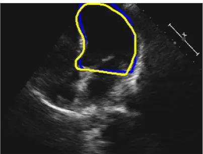
variability, a second operator repeated the LV tracing on 992 frames, blinded to the judgment of the first operator. A typical 2D 4-chamber view is shown in Fig 1, where the locations of manually segmented endocardium by the two operators are highlighted.

Fig. 1. An example 2D 4-chamber view. The blue and yellow curves represent the annotations by Operator-A and Operator-B, respectively.

2.2 Neural network for semantic segmentation

All images were resized to a smaller dimension of 320×240 pixels for feeding into the deep learning models. From the total of 992 images, 595 (60%) were randomly selected for training, 20% of total data used for validation, and the remaining 20% was used for testing.

Standard and well-established U-Net neural network architecture was firstly used since this architecture is applicable to multiple medical image segmentation problems [4]. The U-Net architecture comprises of three main steps such as down-sampling, up-sampling steps and cross-over connections. During the down-up-sampling stage, the number of features will increase gradually while during up-sampling stage the original image resolution will recover. Also, cross-over connection is used by concatenating equally size feature maps from down-sampling to the up-sampling to recover features that may be lost during the down-sampling process.

Each down-sampling and up-sampling has five levels, and each level has two convolutional layers with the same number of kernels ranging from 64 to 1024 from top to bottom correspondingly. All convolutions kernels have a size of (3×3). For down-sampling Max pooling with size (2 × 2) and equal strides was used.

up-sampling, the decoder performs pooling indices computed in the max-pooling step of the corresponding encoder [5]. The number of kernels and kernel size was the same as the U-Net model.

FC-DenseNet model is a relatively more recent model which consists of a down-sampling and up-down-sampling path made of dense block. The down-down-sampling path is composed of two Transitions Down (TD) while an up-sampling path is containing two Transitions Up (TU). Before and after each dense block, there is concatenation and skip connections (see Fig 2). The connectivity pattern in the up-sampling is different from the down-sampling path. In the down-sampling path, the input to a dense block is concatenated with its output, leading to linear growth of the number of feature maps, whereas in the up-sampling path, it is not [6].

Fig. 2. Diagram of FC-DenseNet architecture for semantic segmentation [6].

All models produce the output with the same spatial size as the input image (i.e., 320×240). Pytorch was used for the implementations [10], where Adam optimiser with 250 epochs and learning rate of 0.00001 were used for training the models. The network weights are initialised randomly but differ in range depending on the size of the previous layer [7]. Negative log-likelihood loss is used as the network’s objective function. All computations were carried using an Nvidia GeForce GTX 1080 Ti GPU.

respectively; POA and POB as Predicted LV borders by deep learning models trained

using GTOA and TOB.

3

Evaluation measures

The Dice Coefficient (DC), Hausdorff distance (HD), and intersection-over-union (IoU) also known as the Jaccard index were employed to evaluate the performance and accuracy of the CNN models in segmenting the LV region. The DC (1) was calculated to measure the overlapping regions of the Predicted segmentation (P) and the ground truth (GT). The range of DC is a value between 0 and 1, which 0 indicates there is not any overlap between two sets of binary segmentation results while 1, indicates complete overlap.

𝐷𝐶 =

|𝑃|+ |𝐺𝑇| (1)

Also, the HD was calculated using the following formula for the contour of segmentation where, d (j, GT, P) is the distance from contour point j in GT to the closest contour point in P. The number of pixels on the contour of GT and P specified with O

and M respectively.

𝐻𝐷 = max(𝑚𝑎𝑥𝑗 ∈ [0,𝑂−1] 𝑑(𝑗, 𝐺𝑇, 𝑃), 𝑚𝑎𝑥𝑗 ∈ [0,𝑀−1] 𝑑(𝑗, 𝑃, 𝐺𝑇)) (2)

Moreover, the IoU was calculated image-by-image between the Predicted segmentation (IP) and the ground truth (GT). For a binary image (one foreground class,

one background class), IoU is defined for the ground truth and predicted segmentation GT and IP as

𝐼𝑜𝑈(𝐺𝑇, 𝐼

) =

|𝐺𝑇 ∩ 𝐼𝑃|

|𝐺𝑇 ∪ 𝐼𝑃|

4

Experiment results and discussion

Fig 3 shows example outputs from the three models when trained using annotation provided by Operator-A (i.e., GTOA). The contour of the predicted segmentation was

used to specify the LV endocardium border. The red, solid line represents the automated results, while the green line represents the manual annotation.

U-Net SegNet FC-DenseNet

DC = 0.98 0.96 0.91

HD = 4.24 6 6.78

IoU = 0.99 0.98 0.96

Fig. 3. Typical outputs from U-Net, SegNet, and FC-DenseNet models.

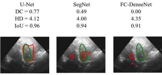
U-Net SegNet FC-DenseNet

DC = 0.77 0.49 0.00

HD = 4.12 4.00 4.35

IoU = 0.96 0.94 0.91

Fig. 4. Failed case example outputs from U-Net, SegNet, and FC-DenseNet models.

Fig 4 illustrates the results for a sample failed case, for which all three models seem to struggle with the task of LV segmentation. By closer scrutiny of the echo images for such cases, it is evident that the image quality tends to be lower due to missing borders, presence of speckle noise or artefacts, and poor contrast between the myocardium and the blood pool.

Table 1. Comparison of evaluation measures of dice coefficient (DC), Hausdorff distance (HD), and intersection-over-union (IoU) between the three examine models, expressed as meanSD.

model DC HD IoU

U-Net _{0.93 ± 0.04 4.52 ± 0.90 0.98 ± 0.01}

SegNet _{0.91± 0.06 4.65 ± 0.89 0.98 ± 0.01}

FC-DenseNet _{0.84 ± 0.11 5.05 ± 0.69 0.96 ± 0.02}

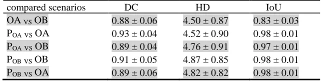
For each image, there were four assessments of the LV border; two human and two automated (trained by the annotation of either of human operators). As shown in table 2, the automated models perform similarly to human operators. The automated model disagrees with the Operator-A, but so does the Operator-B. Since different experts make different judgments, it is not possible for any automated model to agree with all experts. However, it is desirable for the automated models do not have larger discrepancies when compared with the performance of human judgments; that is, to behave approximately as well as human operators.

Table 2. Comparison of evaluation measures (Dice coefficient, Hausdorff distance, and intersection-over-union) for the U-Net model between five possible scenarios.

compared scenarios DC HD IoU

OA VS OB 0.88 ± 0.06 4.50 ± 0.87 0.83 ± 0.03

POAVS OA 0.93 ± 0.04 4.52 ± 0.90 0.98 ± 0.01

POAVS OB 0.89 ± 0.04 4.76 ± 0.91 0.97 ± 0.01

POBVS OB 0.91 ± 0.05 4.87 ± 0.85 0.98 ± 0.01

POBVS OA 0.89 ± 0.06 4.82 ± 0.82 0.98 ± 0.01

5

Conclusion and future work

The time-consuming and operator-dependent process of manual annotation of left ventricle border on a 2D echocardiographic recording could be assisted by the automated models that do not require human intervention. Our study investigated the feasibility of such automated models which perform no worse than human experts.

will examine the correlation between the performance of the deep learning model and the image qualities, as well as using more balanced datasets.

The patients were a convenience sample drawn from those attending a cardiology outpatient clinic. They, therefore, may not be representative of patients who enter trials with particular enrolment criteria or of inpatients or the general population. A further investigation will look at a wide range of subjects in any cardiovascular disease setting. The segmentation of other cardiac views, and using data acquired by various ultrasound vendors can also be considered for a comprehensive examination of the deep learning models in echocardiography.

Acknowledgements

N.A. was supported by the School of Computer Science PhD scholarship at the University of Lincoln.

References

1. Raynaud, C., Langet, H., Amzulescu, M.S., Saloux, E., Bertrand, H., Allain, P. and Piro, P.: Handcrafted features vs ConvNets in 2D echocardiographic images. In: 2017 IEEE 14th International Symposium on Biomedical Imaging (ISBI 2017), pp. 1116–1119. IEEE, Melbourne, Australia (2017).

2. Lang, R. M., Badano, L. P., Mor-Avi, V., Afilalo, J., Armstrong, A., Ernande, L., ... and Lancellotti, P.: Recommendations for cardiac chamber quantification by echocardiography in adults: an update from the American Society of Echocardiography and the European Association of Cardiovascular Imaging.European Heart Journal-Cardiovascular Imaging 16(3), 233-271(2015).

3. Zhang, J., Gajjala, S., Agrawal, P., Tison, G.H., Hallock, L.A., Beussink-Nelson, L., Lassen, M.H., Fan, E., Aras, M.A., Jordan, C. and Fleischmann, K.E.: Fully automated echocardiogram interpretation in clinical practice: feasibility and diagnostic accuracy. Circulation 138(16), 1623–1635(2018).

4. Ronneberger, O., Fischer, P. and Brox, T.: U-net: Convolutional networks for biomedical image segmentation. In: 18th International Conference on Medical image computing and computer-assisted intervention, pp. 234–241. Springer, Munich, Germany (2015). 5. Badrinarayanan, V., Kendall, A. and Cipolla, R.: Segnet: A deep convolutional

encoder-decoder architecture for image segmentation. IEEE transactions on pattern analysis and machine intelligence 39(12), 2481–2495 (2017).

6. Jégou, S., Drozdzal, M., Vazquez, D., Romero, A. and Bengio, Y.: The one hundred layers tiramisu: Fully convolutional densenets for semantic segmentation. In: 30th Proceedings of the IEEE Conference on Computer Vision and Pattern Recognition Workshops, pp. 11–19. IEEE, Honolulu, Hawaii (2017).

7. He, K., Zhang, X., Ren, S. and Sun, J.: Delving deep into rectifiers: Surpassing human-level performance on imagenet classification. In: International conference on computer vision, pp. 1026-1034. Av. IEEE, Santiago, Chile (2015).

9. Jafari, M.H., Girgis, H., Liao, Z., Behnami, D., Abdi, A., Vaseli, H., Luong, C., Rohling, R., Gin, K., Tsang, T. and Abolmaesumi, P.: A Unified Framework Integrating Recurrent Fully-Convolutional Networks and Optical Flow for Segmentation of the Left Ventricle in Echocardiography Data. In Deep Learning in Medical Image Analysis and Multimodal Learning for Clinical Decision Support, pp. 29-37. Springer, Cham (2018).

10. Paszke, A., Gross, S., Chintala, S., Chanan, G., Yang, E., DeVito, Z., Lin, Z., Desmaison, A., Antiga, L. and Lerer, A.: Automatic differentiation in pytorch. In: 31st Conference on Neural Information Processing Systems (NIPS 2017), pp. 1-4, Long Beach, CA, USA (2017).