HAL Id: hal-02533454
https://hal-upec-upem.archives-ouvertes.fr/hal-02533454
Submitted on 6 Apr 2020
HAL
is a multi-disciplinary open access
archive for the deposit and dissemination of
sci-entific research documents, whether they are
pub-lished or not. The documents may come from
teaching and research institutions in France or
abroad, or from public or private research centers.
L’archive ouverte pluridisciplinaire
HAL
, est
destinée au dépôt et à la diffusion de documents
scientifiques de niveau recherche, publiés ou non,
émanant des établissements d’enseignement et de
recherche français ou étrangers, des laboratoires
publics ou privés.
Fully automatic brain tumor segmentation with deep
learning-based selective attention using overlapping
patches and multi-class weighted cross-entropy
Mostefa Ben Naceur, Mohamed Akil, Rachida Saouli, Rostom Kachouri
To cite this version:
Mostefa Ben Naceur, Mohamed Akil, Rachida Saouli, Rostom Kachouri. Fully automatic brain tumor
segmentation with deep learning-based selective attention using overlapping patches and multi-class
weighted cross-entropy. Medical Image Analysis, Elsevier, In press, �10.1016/j.media.2020.101692�.
�hal-02533454�
Fully automatic brain tumor segmentation with deep learning-based
selective attention using overlapping patches and multi-class weighted
cross-entropy
Mostefa Ben naceura,b,∗, Mohamed Akila, Rachida Saoulib, Rostom Kachouria
aGaspard Monge Computer Science Laboratory, Univ Gustave Eiffel, CNRS, ESIEE Paris, F-77454 Marne-la-Vall´ee, France bSmart Computer Sciences Laboratory, Computer Sciences Department, Exact.Sc, and SNL, University of Biskra, Algeria
Abstract
In this paper, we present a new Deep Convolutional Neural Networks (CNNs) dedicated to fully automatic
segmentation of Glioblastoma brain tumors with high- and low-grade. The proposed CNNs model is inspired
by the Occipito-Temporal pathway which has a special function calledselective attentionthat uses different
receptive field sizes in successive layers to figure out the crucial objects in a scene. Thus, using selective
attention technique to develop the CNNs model, helps to maximize the extraction of relevant features from
MRI images. We have also treated two more issues: class-imbalance, and the spatial relationship among
image Patches. To address the first issue, we propose two steps: an equal sampling of images Patches
and an experimental analysis of the effect of weighted cross-entropy loss function on the segmentation
results. In addition, to overcome the second issue, we have studied the effect of Overlapping Patches against
Adjacent Patches where the Overlapping Patches show a better segmentation result due to the introduction of the global context as well as the local features of the image Patches compared to the conventionnel
Adjacent Patches method. Our experiment results are reported on BRATS-2018 dataset where our
End-to-End Deep Learning model achieved state-of-the-art performance. The median Dice score of our fully
automatic segmentation model is 0.90, 0.83, 0.83 for the whole tumor, tumor core, and enhancing tumor
respectively compared to the Dice score of radiologist, that is in the range 74% — 85%. Moreover, our
proposed CNNs model is not only computationally efficient at inference time, but it could segment the whole
brain on average 16 seconds. Finally, the proposed Deep Learning model provides an accurate and reliable
segmentation result, and that makes it suitable for adopting in research and as a part of different clinical
settings.
Keywords: Brain Tumor Segmentation, Class-imbalance, Convolutional Neural Networks, Fully
Automatic, Glioblastomas, Overlapping Patches.
∗Corresponding author.
Email addresses: [email protected](Mostefa Ben naceur ),[email protected](Mohamed Akil ),
1. Introduction
A brain tumor is a growing abnormal cell in the brain or central spin canal (Young and Knopp,2006).
According to the NBTS1, in the United Kingdom, there are more than 4.200 patients with primary brain
tumors (Logeswari and Karnan, 2009). In the United States of America, each year, 13.000 patients die,
and 29.000 patients suffering from primary brain tumors (Singh et al.,2012). Moreover, each patient has a 5
different health condition, age, gender, and a different tumor that could appear anywhere in the brain.
With this huge number of patients in the world and the massive medical data such as device recording,
mag-netic resonance imaging (MRI), positron emission tomography (PET), ultrasound, computed tomography
(CT), X-rays, emerged the need to discover new techniques for the treatment of patients. In addition, the
diagnosis period plays a very important role, especially when we have patients with life-threatening (Schnei-10
der et al.,2010) diseases such as Gliomas tumors, these tumors according to the World Health Organization classification (Gupta and Dwivedi,2017;Louis et al.,2016), have 4 grades (I, II, III, IV). In addition, Gliomas
affect children between 5 and 10 years (Goodman and Fuller, 2014), and adults between 40 and 65 years
(Schneider et al., 2010). Moreover, Gliomas tumors are the most frequent primary brain tumors in adults
(Holland,2001), these tumors represent 81% of all malignant brain tumors (Ostrom et al.,2014), and 45% of 15
all primary brain tumors (Liu et al.,2016). Some patients with Gliomas tumors have survival rate between
0.05% and 4.7% (Ostrom et al.,2014), representing with that the second reason of death. In this paper, our
method is oriented to the segmentation of Glioblastomas (see figure 1) which are brain tumors belonging to
the category of Gliomas tumors.
Figure 1: The four multi-sequence MR images of patients with Glioblastomas tumors. From left to right: Flair, T1, T1c, T2, Ground Truth (GT) labels (created by expert). The color is used to distinguish between the tumor regions: red: Necrotic and Non-Enhancing tumor, green: Peritumoral Edema, yellow: Enhancing tumor, black: Healthy tissue and background. Best viewed in color.
20
Usually, an expert radiologist uses MRI as the most effective (Akram and Usman, 2011; Bhandarkar and Nammalwar,2001) technique to generate Multi-modal images to identify different tumor regions in the soft tissues. Moreover, the radiologist generates four standard MRI images modalities for Gliomas diagnosis
(I¸sın et al., 2016): T2-weighted fluid attenuated inversion recovery (Flair), T1-weighted (T1), T1-weighted
contrast-enhanced (T1c), and T2-weighted (T2) for each patient, then each region of Gliomas tumors needs 25
to be segmented pixel-by-pixel in each slice until the 3D brain volume is divided into meaningful regions as shown in the Ground Truth image (see figure 1). After that, this segmentation map is used for
treat-ment sessions, surgery planning, and follow-up to see if the tumor is growing or shrinking. This procedure
from generating Multi-modal MR images, segmentation, diagnosis, treatment, and follow-up, takes at least
2 months and around 5% of patients stay under this procedure for 5 years (Ostrom et al.,2014). 30
To interpret brain MRI images, a specialized radiologist employs a manual segmentation using information
from MRI images with anatomical and physiological knowledge (I¸sın et al., 2016). Where it’s known that
the manual segmentation in MRI images is a time-consuming and a tedious procedure (Abd-Ellah et al.,
2016). The key challenge is the interpretation and the segmentation of brain MRI images that depend on the expertise of each radiologist (Akram and Usman,2011). Moreover, the mission of radiologist becomes very 35
difficult in the case if the tumor region has intra-tumoral structures such as the Glioblastomas tumors which have three different structures besides healthy tissue inside the tumor region: Necrotic and Non-Enhancing
tumor, Peritumoral Edema, Enhancing tumor (see figure 1). That’s why the Dice score of human rater (i.e.
radiologists) is in the range 74% — 85% (Menze et al.,2015). In addition, the radiologist spends between 3
and 5 hours (Kaus et al.,2001) to extract features manually from MRI images then to label each pixel if it 40
belongs to a tumor region and which region from 3 regions or it belongs to healthy tissue. Thus, the manual
segmentation is a time-consuming compared to automated methods which take between few seconds and
20 minutes using GPU implementation. Since the aim is to obtain a segmentation of brain tumors, given
the number of patients, obviously fully automated segmentation methods are practical for day-to-day use in
clinical centers and for research. 45
After the breakthrough in 2012 in the field of computer vision where a team developed a deep learning model called AlexNet (Krizhevsky et al., 2012), this model outperformed the state-of-the-art methods and
it achieved the best result in the field of object recognition. Since 2014, many deep learning-based research
(Ben naceur et al., 2018; Havaei et al.,2017; Pereira et al., 2015) have been proposed in the field of brain
tumor segmentation. Also, in the last decades, we noticed that the number of published papers involving 50
brain tumor segmentation increased exponentially (Menze et al.,2015), this increase indicates that creating
a Computer-Aided Diagnosis (CAD) (Akram and Usman,2011;El-Dahshan et al.,2014) has always been a
highly needed option and necessary (Zhang et al.,2001). In addition, some patients have aggressive tumors
that need to be treated in less than two months. This CAD system could decrease the needed time for the
diagnosis process (El-Dahshan et al., 2014) and it could give to Oncologists more time with their patients 55
in the process of treatment and follow-up.
The addressed problem in this paper is how to obtain the most accurate and reliable brain tumor
in addition to Healthy tissue: Necrotic and Non-Enhancing tumor, Peritumoral Edema, Enhancing tumor,
where also Gliomas, including Glioblastomas, invade the surrounding tissue rather than displacing it, causing 60
unclear boundaries, moreover, Gliomas in MRI images have the same appearance as Gliosis, stroke,
inflam-mation, blood spots (Goetz et al.,2016), to solve this problem, we propose a CNNs model that is inspired
by the Occipito-Temporal Pathway (OTP), this structure made up of many sub-regions (V1, V2, V4, IT)
(Desimone et al.,1989). The design of our CNNs model allows to maximize the features’ representation of
Glioblastomas tissue, also leads to detect and predict even small regions with fuzzy borders. 65
(ii) The second challenge is the Artificial Neural Networks, including CNNs, do not perform well with highly
unbalanced data such as BRATS dataset where 98% of data (Havaei et al., 2017) are healthy tissue (i.e.
non-tumorous). The training of CNNs architecture with unbalanced data, will make predictions with low
sensitivity, thus the CNNs architecture will bias toward the healthy class. In medical applications, the most
important metric for a clinical decision support system is sensitivity (Hashemi et al.,2018) toward tumoral 70
regions. Thus, to overcome this problem, we conduct many class-weighting evaluations (see section 3.4) by
adding weights to the loss function. Like this, we can adjust the contribution of each output by a specific
weight, which has been shown to be effective for image segmentation (Badrinarayanan et al.,2015) and for
the problem of unbalanced medical data such as brain tumor segmentation (see section 3).
(iii) The third challenge is common in semantic image segmentation problem, where this challenge is about 75
the reduction of features during the pooling layers and convolution striding (Chen et al.,2017). To treat this
challenge, we use short and long skip connections (Drozdzal et al., 2016; He et al., 2016) which encourage
the reuse of low-level features such as lines, edges. The combination of low-level features with high-level
features such as shapes, objects helps CNNs architectures to better locate the boundaries of tumor regions.
(iv) The fourth challenge is to make the prediction more accurate by solving the limitation of segmentation 80
methods that are based on image Patches; it’s known that CNNs do not take into account the relationship
among image Patches (Zhao et al.,2018). In our work, Overlapping Patches is used to extract more Patches
in the intersection of Adjacent Patches. Like this, we can extract global features such as the relationship
among Patches and their positions in the entire brain image, as well as local features such as pixel intensity
and pixel label. Through this work, we developed an End-to-End framework for brain tumor segmentation 85
based on a new inspired CNNs architecture. To the best of our knowledge, this work is the first work succeed
to address these four challenges together.
In this paper, our goal is to propose and develop an End-to-End Deep Convolutional Neural Networks model
for fully automatic brain tumor segmentation. The proposed model is used to segment the brain tumors of
Glioblastomas with both high- and low-grade. For achieving this goal, we propose four contributions: 90
1. First we propose a new Deep Learning model with 3 variants architectures which give more accurate
state-of-the-art methods. Details of these contributions are dedicated to address the first and the third
challenges.
2. To overcome the unbalanced data problem, we studied the effect of class-weighting technique on CNNs 95
segmentation results, where we propose a set of weights for the 4 sub-regions. Moreover, details of this
technique in section 3.4are oriented to treat the second challenge.
3. We propose also Overlapping Patches technique to improve the segmentation results, i.e. the use of
Adjacent Patches help to extract local features, but the use of Overlapping Patches helps to use small
Patches and to extract both local and global features. The Overlapping Patches allowed us to handle 100
the fourth challenge (in section 3.2).
4. Our CNNs model is a very fast model, also it could segment the whole brain on average 16 seconds,
i.e. reducing the number of parameters and using small Patches through Overlapping Patches helped
to reduce the training and the inference time.
After reviewing the state-of-the-art in the field of brain tumor segmentation, machine learning based 105
methods, and the current CNNs-based methodsin section 2. Then, we explain our approach for solving the
problem of brain tumor segmentation in section 3. Then, we describe BRATS dataset and the evaluation
metrics, also the results of our approach in section 4. Finally, the conclusion and the perspectives are
describedin section 5.
2. Related work
110
Most research on Pattern Recognition and Machine Learning from 1970s to 1990s: were based on features
engineering (i.e. hand-designed features) and mathematical models, in which the researchers use training
data to extract the input (binary or real) vector of features, then the research in 1990s to 2000s jumped
to use less feature engineering and more discriminative models which use a lot of data to extract several
features then using a classifier at the end of the pipeline to distinguish between the different classes. These 115
classical approaches are in overall: threshold-based methods (Gibbs et al., 1996; Stadlbauer et al., 2004),
Region-based methods (Cates et al., 2005; Kaus et al., 2001), Edge-based methods (Caselles et al., 1993;
Lefohn et al., 2003), Atlas-based methods (Menze et al., 2010; Prastawa et al., 2003), Classification and Clustering methods (Bhandarkar and Nammalwar, 2001; Clark et al., 1998; Fletcher-Heath et al., 2001).
These methods generally produce poor results and need a user interaction (e.g., region growing) most of 120
the time and sensitive to noise (e.g., edge detector). Moreover, they needprior knowledgefrom experts and
feature engineering. Also, they are in overall computationally expensive and use a lot of memory due to
computing a huge number of features.
In 2006, appeared a new type of learning method called Deep Learning which uses a huge number of data
to extract many low-features such as lines, edges with different orientations then it combines them in a 125
hierarchical way to obtain high-level features such as shapes, objects, and faces. Moreover, the research on
tumor segmentation or lesion segmentation in overall with Deep Learning started in 2014.
(Havaei et al.,2017) proposed a fully automatic brain tumor segmentation method based on Cascaded
Con-volutional Neural Networks which are an extended version of the work (Axel et al.,2014), these Cascaded
Networks used two pathways that are trained in different phases to capture local and global features. They 130
used also as input 2D Axial Patches with four MR sequences as channels where each pathway has a different
input patch size. Moreover, they proposed two stages of training for the problem of class-imbalance to
correct in the second training stage the Patches that are biased toward the wrong class. After that, they
applied a threshold technique as a post-processing method to remove the connected-components near to the
skull. In addition, this Cascaded architecture takes 180 seconds to segment the complete brain using GPU 135
implementation (Havaei et al.,2017).
(Chang,2016) developed a CNNs model that is based on two concepts (1) a fully convolutional architecture that predicts a dense output matrix size as used in the original input (Long et al., 2015), (2) Hyperlocal
features concatenation; the input MR images is re-introduced in the concatenation layer before the output.
This technique is used first by (Yang and Ramanan, 2015) in their architecture Directed-Acyclic-Graph 140
which is a new variant of standard CNNs (LeCun et al., 1998). The architecture of (Chang, 2016) has 7
convolution layers in addition to upsampling and concatenation layers. In this CNN architecture, 4 channels
of MRI images are used as an input (i.e., Flair, T2, T1c, T1). Moreover, this architecture takes 0.93 seconds
to segment the entire brain using GPU implementation (Chang,2016).
(Ellwaa et al.,2016) proposed an iterative method which is based on a random forest with 100 trees, each 145
of which has depth 45, their method extracts 328 features from MRI images, these features are gradient
features, appearance features, and context-aware features. The input to their method is 4 channels of MRI images (i.e., FLair, T1, T1c, T2). This iterative method works by choosing in each iteration 5 patients and
add them to the training set, then they continue the training of this random forest until the training set
reaches 50 patients, where at 50 patients their iterative method stops. 150
(Kamnitsas et al., 2016, 2017) developed a 3D-CNNs model for brain tumor segmentation based on the
model’s performance (Urban et al., 2014). These 3D-CNNs networks composed of dual pathway with 11
layers, the input to this network is 3D MRI images (i.e. Flair, T1, T1c, T2), also each pathway has a
differ-ent input patch size (i.e. 4×253,4×193). Then, they added conditional random field as a post-processing operation to remove mis-classification regions and as a spatial regularization. Moreover, they extended their 155
network with residual connections (He et al.,2016), in which this new extended network (Kamnitsas et al.,
2016) did not obtain a big improvement compared to the original model (Kamnitsas et al.,2017). Their 3D CNNs model takes 24 hours for training using GPU implementation, and for testing, it takes 35 seconds to
(Zhao et al., 2018) developed a brain tumor segmentation method based on the integration of CNNs and 160
conditional random field in one network, as opposed to (Kamnitsas et al.,2017) who used conditional random field as a post-processing step. The authors of (Zhao et al.,2018) developed 3 CNNs networks that take as
an input 3 types of MRI images (i.e., Flair, T1c, T2). Each of these 3 networks use two pathways similar to
(Havaei et al.,2017; Kamnitsas et al., 2017), where these pathways are trained on 2D image Patches (i.e.,
33 × 33 and 65× 65) and slices (i.e. 240 × 240) from axial, coronal and sagittal views. For the testing 165
step, the prediction results from 3 views are fused using a voting strategy. Moreover, these 3 networks took
12 days for training using GPU implementation, and for testing, each model took for each view (i.e., axial,
sagittal, coronal) on average 3 minutes to segment the entire brain, i.e., 3 networks×3 minutes in addition to fusion time which is not reported in the original paper.
In a previous work (Ben naceur et al.,2018), we proposed 3 fully automatic brain tumor segmentation meth-170
ods, where we achieved the state-of-the-art performance. The proposed methods are based on the concept of incremental optimization; after one cycle of training, a new block is added automatically on top of last
blocks. The followed strategy in this work is based on 2 rules (1) as we add more layers, we get a better
segmentation performance, (2) after many experiments to form one block, we found that deep learning
mod-els that are based on 2 or 3 consecutive layers of convolution provide a good segmentation performance. 175
This new strategy called automated machine learning (AutoML) (Zoph et al., 2018;Pham et al.,2018), is
a new field of artificial intelligence; AutoML attempts to design new machine learning models without the
intervention of users. The proposed segmentation methods are trained on 2D image Patches (32×32) that are extracted from the Axial view. The training time took≈5 hours and the testing time took in range 19 -21 seconds to segment the entire brain tumor using GPU implementation. The limitation of this method is 180
the GPU memory; where after a certain training time, the memory gets overwhelmed by the added blocks. To overcome this issue, we replaced in this paper the added blocks by a new concept called modules. These
modules are inspired by the interconnection among the brain’s regions: retina, V1, V2, V4, IT.
(Mlynarski et al.,2019) developed a fully automatic brain tumor segmentation method based on a
combina-tion of six models of 3D Convolucombina-tional Neural Networks (CNNs) architectures. Each of these architectures 185
is composed of three (or five) CNNs architectures, also, these architectures are trained independently and
dedicated for one MRI view (e.g. Axial, Coronal or Sagittal slices of the input image) and one architecture
based on 3D CNNs. The proposed segmentation 3D CNNs model is trained on channels concatenation
be-tween extracted feature maps from the Axial, Coronal and Sagittal dedicated architectures and two (T2 ,
T1c) or four (T2, T2-Flair, T1, T1c) 3D multisequence MR images. The technique of using feature maps 190
as an additional input into the architecture of another CNNs, is used by (Havaei et al., 2017). Moreover, (Mlynarski et al., 2019) addressed two issues: the first one is long rang context, to solve this issue, they
the receptive field. The second issue is unbalanced data, where they solved this issue by using weighted
cross-entropy as a loss function. 195
2.1. Related work discussion
As a summary of related work, the cited works (Chang, 2016; Ellwaa et al., 2016; Havaei et al., 2017;
Kamnitsas et al.,2017;Zhao et al.,2018;Ben naceur et al.,2018;Mlynarski et al.,2019) address the main problem of fully automatic brain tumor segmentation in different ways. In addition to the main problem, there are three important subproblems: (1) unbalanced data; the class of interest (i.e. tumoral region) has 200
the minority of labels which represent for example in our dataset almost 2% of data, while the healthy class
has 98% of data. This subproblem is solved by two training step (Havaei et al., 2017), equal sampling of
training patches (Havaei et al., 2017; Zhao et al., 2018), weighted cross-entropy (Mlynarski et al., 2019),
Online Class-Weighting Approach (Ben naceur et al., 2019), (2) long-range context modeling (e.g., tumor
shape, relationship between tumor parts, spatial dependencies) using all pixels in the same 2D slice, as 205
opposed to the short-range 3D context that is computationally expensive. In this case, to achieve the
trade-off and to benefit from 3D context through 3 views (i.e., Axial, Coronal, and Sagittal), thus using small 3D
patches is the best solution. In images segmentation applications, short- and long-range context modeling
could enhance CNN’s capability to distinguish pixels, especially those at the borders. The subproblem of long-range context is solved by (Mlynarski et al.,2019), also this subproblem is solved partially by (Chang, 210
2016;Havaei et al., 2017; Zhao et al., 2018;Ben naceur et al.,2018). Moreover,one of the important sub-problems in CNNs is (3) the relationship among patches (also known as modeling the patches in images), because the training method typically used in CNN is patch-by-patch, we refer to this method as Adjacent Patches. The limit of Adjacent Patches is that it does not take into consideration (Havaei et al.,2017;Zhao et al., 2018) that the set of patches (e.g., each patch has 64 x 64) represents the full image (in our case 215
240 x 240). The issue of modeling both context and spatial relationship in image segmentation is solved by multi-scale (multi-resolution) approach (Kamnitsas et al., 2017), we also solved this issue by using our proposed Overlapping Patches approach (see section 3.2).
In this paper, we developed new CNNs architectures from scratch, these architectures are able to detect effectively the tumoral regions. Also, we addressed many issues such as unbalanced data and the spatial 220
relationship among patches, also we solved partially the issue of long-range context. The first issue (i.e.,
unbalanced data) is addressed using the class-weighting technique, and the second issue is solved using
Overlapping Patches technique. In addition, we choose the best four positions in a MRI image to extract the
most relevant features with the minimum patches. The third issue (i.e. long-range context) is solved partially
using Axial MRI images (i.e. 2D Axial slice) to reduce the computational cost of the CNN’s parameters 225
in addition to reduce the training and the inference time. Consequently, the solved issues allowed us to
In this study, we have been motivated by the success of deep learning in computer vision and in the context
of brain tumor segmentation. From 2014 until now, the brain tumor segmentation performance has been increased a lot and the inference time of fully automatic methods has been decreased dramatically from≈ 230
20 minutes to few seconds. Here besides the functionality of CNNs, we propose deep learning architectures
inspired by the visual cortex structure to model the function and the structure of biological neural networks.
These architectures are trained using MRI image Patches extracted from the axial view. Moreover, to avoid
the class-imbalance problem, we apply two techniques: the number of training Patches is equally extracted
for each class, and a new class-weighting technique is proposed. In addition, we have also studied the effect 235
of Overlapping Patches on deep learning performance in order to solve the issue of brain tumor segmentation
methods that are based on image Adjacent Patches. The novelty of our architectures is: (1) the efficiency
in terms of inference time and in terms of memory by removing fully connected layers and replacing them
by Fully Convolutional Networks (Long et al., 2015), (2) our analysis of the blocks technique (Ben naceur et al.,2018), led us to replace this technique by the concept of modules that showed an improvement of the 240
boundary delineation. In addition, (3) the solved issues (i.e. unbalanced data, relationship among patches)
allowed this pipeline to reach the state-of-the-art performance.
3. Proposed brain tumor segmentation method
The proposed brain tumor segmentation pipeline has three stages: pre-processing, then segmenting the
Overlapping MRI Patches using CNNs-based architectures, and finally two post-processing techniques. 245
3.1. Pre-processing
To remove some noises and to enhance the quality of MRI images, especially the MRI images of the
BRATS dataset are generated using different MRI devices and acquisition protocols. Thus, to mitigate the
issue of different intensity ranges among the BRATS’s images, we applied 3 pre-processing steps based on
this work, and on (Ben naceur et al.,2018). Our normalization method of each 2D axial image (i.e. a slice) 250
is as follows:
1. Removing 1% highest and lowest intensities: this technique helps to remove some noises at the tail
of the histogram, where this step has provided good results in many research (Havaei et al., 2017;
Tustison,2013).
2. Subtracting the mean and dividing by the standard deviation of non-zero values in all channels: this 255
technique is used to centre and to put the data in the same scale, i.e., bringing the mean intensity
value and the variance between one and minus one.
3. In this step, we try to isolate the background from the tumoral regions by assigning the minimum
architectures. The application of the second pre-processing step, led to bring the mean value in the 260
range [-1, 1], in other words, the intensities of all regions in addition to healthy and background became between -1 and 1. As we know, the intensity of background pixels of MRI images in BRATS data equals
to 0, thus to isolate the zero pixels (i.e. background) from the other regions, we normalized histogram
of the MRI images by shifting the zero pixels to another bin outside the range [-1, 1]. We found that
the bin -9 in many experiments, gives good results in the training and testing phases. 265
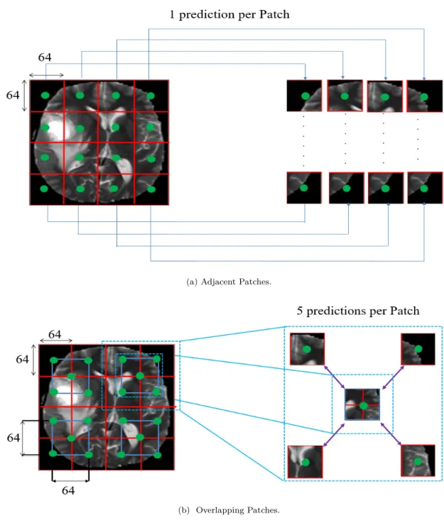
3.2. Overlapping Patches
Our CNNs architectures are built upon 2D image Patches, in which these architectures predict the pixel’s
class which is the center of the 2D Patch (i.e. see figure 2, green points). A lot of research (Urban et al.,
2014;Pereira et al.,2015;Havaei et al.,2017;Ben naceur et al.,2018) use the technique of Adjacent Patches (see figure 2.a), i.e. using Patches (Patch is a set of pixels) that are next to each other, but the limit of CNNs 270
with Adjacent Patches is that CNNs do not take into account the fact that these Adjacent Patches together
make up the entire image (Havaei et al., 2017; Pereira et al., 2017; Zhao et al., 2018). Thus, to overcome
this problem and to make the CNNs architectures more accurate, we extract Overlapping Patches (see figure
2.b) which help these architectures to see the local (Red Patches,see figure 2.b) and the larger context (Blue Patches,see figure 2.b). It is well-known that CNNs work by convolving each kernel with the corresponding 275
Patch in the image, then this kernel moves to the next Patch to complete the entire image. Then through
the learning process, the CNNs will attempt to classify these adjacent Patches into different classes (i.e., 4
sub-regions), so the final segmented image will be the result of only one pixel prediction (i.e., green point)
per Patch as shown in figure 2.a. However, with the Overlapping Patches, the final segmented image will
be the result of 5 predictions per Patch as shown in figure 2.b, where the prediction of the other 4 pixels 280
affects the prediction of the first pixel and vice versa for each pixel. Thus with the technique of Overlapping
Patches, CNNs could learn to build a relationship among these Patches (Red Patches,see figure 2.a). So,
when applying CNNs architecture with the technique of Overlapping Patches, the architectures still able to
classify and see the larger context even using small Patches. The explanation of why Overlapping Patches
provide more accurate results than Adjacent Patches is due to the prediction of each pixel’s label comes 285
from its neighborhoods. Thus, using different Patches around the same pixel, the final decision (i.e. final
prediction) of that pixel’s label will be based on the vote of the majority of decisions, in other words, the
final decision will come from 5 other pre-decisions. In addition, the use of Overlapping Patches provide a
data augmentation (Hashemi et al.,2019) of the original BRATS dataset through a better balance of training
dataset. 290
(a) Adjacent Patches.
(b) Overlapping Patches.
Figure 2: Examples of A) Adjacent Patches (one prediction per Patch) and B) Overlapping Patches (5 predictions per Patch) from an input MRI image. The training dataset is created by extracting Overlapping Patches (i.e. Red and blue boxes). Best viewed in color.
3.3. Model and Architectures
MRI provides images that show a contrast between the soft tissue of the brain (or other human organs
such as liver) (Akram and Usman, 2011; El-Dahshan et al., 2014), in which these images in many times
do not clearly show the border between brain regions, where the brain appears as a single mass. Thus, to
extract only the tumoral regions from the whole brain, the proposed model should extract more features 295
about the healthy tissue and the tumoral regions. To solve this issue, we propose three CNNs architectures
that are based on the question of how to maximize the features’ representation inside the model, in other words, how to extract much relevant features (Ghebrechristos and Alaghband,2018) from MRI images.
3.3.1. Visual areas-based interconnected modules
Developing a CNNs architecture based on the rule of using many interconnected modules, is known in 300
the state-of-the-art and it provides a good performance in many applications such as GoogleLetNet model
(Szegedy et al.,2015) that is built based on the module of Inception, ResNet model (He et al., 2016) which
is based on many modules of residual layers, 3CNet (Ben naceur et al., 2018) is built also on the system
of modules. Moreover, the structure of OTP is built on the rule of interconnected areas (i.e. modules):
V1, V2, V4, IT (Manassi et al., 2013). Thus, following this rule of interconnected modules, we build our 305
CNNs architectures, where we build first two modules called Sparse Connection OCM (OCM: OCcipito
Module) and Dense Connection OCM, these two modules are based on the structure of OTP, this structure
is important and critical for object recognition (Desimone et al.,1989) and for the brain’s memory (Kl¨ uver-Bucy syndrome (KBS), experiments of Kl¨uver and Bucy 1937) (Ono and Nishijo,1992).
The algorithm of CNNs (LeCun et al.,1989,1998) originally is inspired by the visual system. In 1962, Hubel 310
and Wiesel (Hubel and Wiesel, 1962) discovered that each type of neurons in the visual system, responds
to one specific feature: vertical lines, horizontal lines, shapes ...etc. From this discovery, the algorithm of
Neocognitron is developed (Fukushima and Miyake, 1982), but the problem of Neocognitron is: does not
have a supervised learning algorithm (LeCun et al., 2015), where in CNNs they solved this problem by
using Backpropagation algorithm (Rumelhart et al., 1986). Moreover, we find that the visual system has 315
a specific structure that is composed of several visual areas: V1, V2, V4, IT (Manassi et al., 2013). As
we said before, CNNs is inspired by the visual system function, what was the ”missing part” of CNNs is
the architecture’s structure. Thus, in this work, we attempt to inspire from the visual system its internal structure. By inspiring the structure of the visual system, we could add to the function of CNNs a specific
architecture. 320
To determine a shape in the visual system, for example, a person’s face, it will be processed from lines
and edges at V1 area to shapes at V2 area to objects at V4 area to faces at the end at IT area (Herzog and
Clarke, 2014; Manassi et al.,2013). Thus, the OTP structure has four properties (i.e. N:1 to N:4): 1. Retina is the input of the visual system.
2. The visual cortex treats the forms hierarchically; object has different shapes, and shape has different 325
lines and edges and so on.
3. OTP structure is composed of several interconnected visual areas (i.e. V1, V2, V4, IT), where each
area responsible for a specific task.
In our work, we attempt to build a CNNs model inspired by the OTP structure, thus, we inspired: 330
1. The Retina represents the input images.
2. The hierarchical function using convolution operators.
3. We have developed two modules inspired by the area V1 and V2, interconnected to each other using
direct and skip connections (see section 3.3.2.1).
4. To take into account the last property (N: 4) of visual cortex, there are two ways: 335
(a) Reducing the feature maps at each level using Pooling operation.
(b) Or using larger kernels at each convolution layer incrementally.
The use of larger kernels (i.e. the property (4.b)) increases the computational time (i.e. increase the
number of operations), on the other hand, the use of small kernels, has proved previously that they keep a
lot of information and it allows the CNNs model to be deeper in terms of layers (Simonyan and Zisserman, 340
2014a). Thus, from the above explanations, we will use the first option (i.e. 4.a).
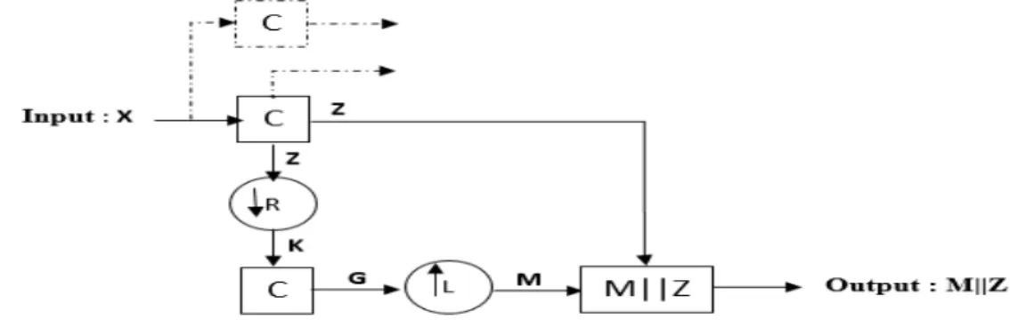
3.3.1.1 Building the first module V1
In this work, we consider the structure of V1 is the same as V2, V4, IT, but the output of these modules
is different from module (e.g. V1) to another (e.g. V2). Thus, the module of V1 is composed as shown in
figure 3 of: an input (phase 1), then we have convolution layers (phase 2), and a max-pooling layer (phase 345
3), then another convolution layers (phase 4), upsampling (phase 5) and concatenation layers (phase 6):
Figure 3: An illustration of visual area V1. C is a convolution operator, Z and G are feature maps, K is the output of Pooling layer, M is a high-resolution feature map,↓Ris a pooling layer,↑Lis an upsampling operator,M||Zis a concatenation layer between M and Z. Also, the continuous lines are direct and skip connections, and dashed lines are used to build the second module of visual area V1 (i.e. DenseConnectionOCM).
1. First phase: let’s consider the Retina as the input (i.e. X) to our model.
2. Second phase: obtaining a hierarchical structure is guaranteed by the method of convolution operation;
convolution uses a filter bank (i.e. trainable parameters) to extract many levels of features across the
entire input images. Moreover, from our previous work (Ben naceur et al., 2018), we found that 350
using two consecutive convolution layers with kernel size equals to 3×3 provides a high performance. Thus, in this work we will use two consecutive convolution layers Z = Conv(Conv(X)). The output of convolution layer called feature maps Z which are calculated as follows (see equation 1):
U =bi+ m
X
j=1
Wij∗V (1)
WherebiandWij (i, j∈N) are trainable parameters, called respectively bias and weights. m is the size
of the input (m∈N). V and U are respectively input and output, and ’*’ is the convolution operation.
355
After that we apply a non-linear activation functionRelu(U) =max(0, U). In CNNs architecture,Wij is the kernel parameters.
3. Third phase: to reduce the feature maps dimensionality (as described in property N: 4), we use
Max-Pooling 2 ×2 operation to provide the minimum reduction of feature maps in addition to the shifting 360
invariant property. Max-Pooling takes the maximum value of each non-overlapping square (i.e.
sub-region) of feature map Z. MaxPoolingKij is computed as follows (see equation 2):
Ki,j= max
h Zi+h,j+h (2)
Whereh∈Nis the size of sub-region,i, j∈Nare the stride values for the vertical and horizontal axes
respectively.
4. Fourth phase: using trainable parameters G = Conv(Conv(K)) again to extract more feature maps 365
from the Max-pooling output. Also, to compute the feature maps G, we useequation 1:
5. Fifth phase: to concatenate two types of features maps (i.e. feature maps of phase 2 and phase 5),
where these two types of feature maps are not at the same scale. Thus, to obtain higher-resolution
feature maps from lower-resolution feature maps in CNNs architecture, there are two techniques: (1)
deconvolution, (2) upsampling. The first one uses trainable parameters, but the second technique 370
does not use any trainable parameters, this technique works by inserting zeros padding internally
between pixels, where the number of zeros is determined by the stride parameter. The final step is
to convolve the sparse feature maps with trainable parameters (i.e. convolution operation) to obtain dense features maps, this technique helps to avoid the problem of Overfitting (Badrinarayanan et al.,
2015). The method of upsampling operator works as follows (see equation 3and4): 375 ML[n] =G(n)↑L Mi(n) =upsamplingL,n(Gi) (3) Mi= Gi(n/L) , if(n/L)∈ N 0 , otherwise (4)
Upsampling operator works by insertingL−1 zeros betweenG(n) andG(n+ 1) for allnelements.
6. Sixth phase: is the concatenation layer, where in this layer, we concatenate the feature maps of phase
2 and phase 5.
We used the phases from 1 to 6 to build a Sparse Connection OCM module (see figure 4.a), and a Dense 380
Connection OCM module (see figure 4.b), while in the second module (i.e. Dense Connection OCM module),
we have added 1 × 1 convolution layer (Lin et al., 2013) which operates over N-dimensional volumes and also it’s considered as a preliminary classification of the input images. Dense Connection OCM and Sparse
Connection OCM modules are two representations of the visual area V1, in which from these two modules, we have deduced three CNNs architectures (see section 3.3.2.2). The motivation of these two modules is 385
they attempt to model the structure of OTP, moreover these modules extract different representations from
the input MRI images where this technique is used by GoogleLetNet in its Inception module (Szegedy et al.,
2015). We have used two different types of convolution operations (i.e., 3×3 and 1×1) for the module Dense Connection OCM and Sparse Connection OCM to diverse the feature representations of the MRI images:
• Sparse Connection OCM module: applies a strategy of sparse connectivity, where we connect a subset 390
of convolution layers to each other. This module has one input and two outputs (i.e. output 1 and
output 2). We refer to this module as SparseConnectionOCM. The details are illustratedin figure 4.a.
• Dense Connection OCM module: applies two strategies (1) Dense connectivity and (2) 1 ×1 convo-lution operation, where we concatenate all high-level feature maps and low-level feature maps in the
concatenation layer before the output. This module has one input and one output compared to the 395
previous module (i.e., Sparse Connection OCM). We refer to this module as DenseConnectionOCM.
The details are illustratedin figure 4.b.
3.3.2. CNNs architectures
To connect between different modules of CNNs architecture, we use two types of connections: first a
direct connection from layerHL−1 to layer HL through a mapping non-linear function f (see equation 5), 400
secondly a special type of connection called skip connection that connect layerHL−i to layerHL(see section
3.3.2.1).
HL=WL×HL−1+bL (5)
Where bL, WL are trainable parameters, called respectively bias and weights, after that a non-linear
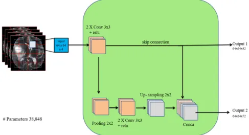
(a) SparseConnectionOCM, where we use a skip connection to connect between low-level feature maps and a pre-output concatenation layer. This module has 38,848 parameters.
(b) DenseConnectionOCM, where we use multiple skip connections to connect data and low-level feature maps and pre-output concatenation layer together. This module has 48,100 parameters.
Figure 4: Schematic representation of the SparseConnectionOCM and DenseConnectionOCM. Each orange/purple/yellow box corre-sponds to multi-channel feature maps. The input represents the multi-modal MRI images. Each output (i.e. output 1, output 2, and output) is an input to the next module. Conv is the convolution operator, 1×1 and 3×3 are the filter’s size, pooling 2×2 is the max-pooling operator with 2×2 window. Relu is the non-linear activation function, upsampling is the upsampling operator, Conca is the concatenation layer, skip connection is a connection between two non-successive layers.
3.3.2.1 Skip connections
405
The use of skip connections is very important; it helps to backpropagate the gradient signal across several
Skip connections have been shown an improvement of accuracy for many computer vision tasks compared
to the state-of-the-art methods. For example in the field of biomedical image segmentation (Drozdzal et al., 2016) such as U-net (Ronneberger et al.,2015), and Fully Convolutional Networks (FCN) were applied for 410
semantic segmentation (Long et al., 2015), also for image recognition such as ResNet (He et al., 2016),
ResNext (Xie et al., 2017), DenseNet (Huang et al., 2017). The use of skip connections encourage the
architecture to reuse the features especially low-level features such as lines, edges; the model uses these
low-level features many times with high-level features such as shapes, objects at the same level. Thus, the
combination of low-level features and high-level features in MRI images using skip connections, helps to 415
localize the tumor region and then to detect the shape and the boundaries of intra-tumoral structures (i.e.
4 sub-regions). Skip connections connect between two non-successive layers: layerHL−i and layerHL (see
equation 6):
HL=WL×HL−i+bL (6)
WherebL,WLare trainable parameters, called respectively bias and weights. HL−i,HL (i∈
N& 2≤i)
are two layers, after that a non-linear activation functionf(HL) is applied. 420
3.3.2.2 Sparse and Dense architectures
CNNs are known for its ability to extract many complicated and hierarchical features from images, thus, to develop a deep CNNs architecture, we have either pixel-wise approach or patch-wise approach. In the first
approach, CNNs deal with Pixels, while in the second approach, CNNs deal with Patches. Our method in
this paper is based on Patch-wise technique, thus CNNs architecture takes as input patches with limited 425
size (in our case 64 x 64), where the size of patches is lower than the size of the full image (240 x 240). The
training data is a set of Patches, each 64 x 64. CNNs treat the generated patch, patch-per-patch until the
end of pre-defined number of patches, moreover, for each patch, there are three other patches as channels
for the multi-sequence of MRI images. The most used technique to generate patches is adjacent patches (see
figure 2.a). Then, at prediction time, CNNs predict the segmentation labels separately from others (Havaei 430
et al.,2017); the labels of second patch will be predicted without any relation with the first patch and so on for third, fourth ...etc. In literature, methods such as K-means (Zhang et al., 2019) or conditional random field (Wu et al.,2014), are defined over all pixels or all labels of the full image, like this, the prediction of a
label is shared among all pixels, or labels through a proximity distance or a mean-field message respectively.
Thus, the patch-wise technique is based on adjacent patches with limited size. From the other hand, to 435
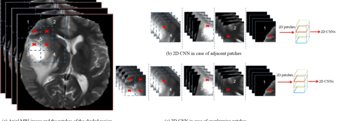
overcome the issue of adjacent patches, we create a link among all these patches of the entire image, where
we proposed overlapping patches (see figure 2.b) technique; it works by constructing a new patch by taking
patch) is a shifting of each patch (from the remaining four patches) horizontally and vertically on the width
axis, then on the height axis respectively (see figure 5). Secondly, we proved through a series of experiments 440
on adjacent patches and overlapping patches, and we found that training CNNs architecture with overlapping
patches, provides a good segmentation performance in terms of dice score complete, core, enhancing and
average dice compared to adjacent patches (see table 2, and figure 7). Moreover, pixel-wise classification in
Figure 5: Examples of (a) a MRI image (Axial view) and the patches of the shaded region, where the red cross signe represents the shared region with the patch number 5. (b) 2D CNNs in case of Adjacent Patches: at each epoch of training we use only 4 patches at the shaded region. (c) 2D CNNs in case of Overlapping Patches: at each epoch we use 4 patch in addition to a new patch (number 5) constructed from the four patches. Best viewed in color.
CNNs is computationally expensive such as the architecture of AlexNet (Krizhevsky et al.,2012), VGGNet
(Simonyan and Zisserman,2014b). From another side, Fully Convolutional Networks (FCN) (Ronneberger 445
et al.,2015;C¸ i¸cek et al.,2016;Milletari et al.,2016) have shown a great performance. FCN approach is based on patch-wise classification and it has shown better and more accurate results than pixel-wise classification.
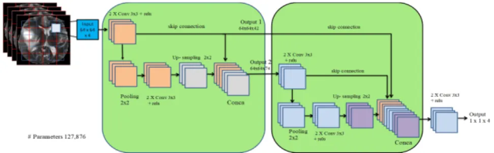
In this work we investigate three variants of CNNs architectures:
• Sparse MultiOCM architecture: this architecture made up of two modules of SparseConncentionOCM which has two outputs (i.e. output 1 and output 2), we concatenate the first output (i.e. output 1) 450
with a pre-output concatenation level (i.e. conca layer) of the second module, and the second output
(i.e. output 2) is used as an additionnel input to the second module. We refer to this architecture as
SparseMultiOCM. The details of this architecture are illustrated in figure 6.a.
• Input Sparse MultiOCM architecture: this architecture is the same as SparseMultiOCM, where the difference is: in this architecture we investigate the effect of adding directly the input as another 455
concatenation feature maps. We refer to this architecture as InputSparseMultiOCM. The details of
(a) SparseMultiOCM, we use two modules of SparseConnectionOCM to build this archi-tecture. This architecture has 127,876 parameters.
(b) InputSparseMultiOCM, we concatenate the input with the pre-output concatenation level in two modules. This architecture has 130,180 parameters.
(c) DenseMultiOCM, we use two modules of DenseConnectionOCM to build the complete architecture. This architecture has 181,124 parameters.
Figure 6: An illustration of the proposed CNNs architectures to solve the problem of fully automatic brain tumor segmentation. Each orange/red/purple/yellow box corresponds to multi-channel feature maps. The output 1×1×4 is a 1×1 convolution layer with 4 classes of BRATS dataset where we have 4 sub-regions: Healthy tissue, Necrotic and Non-Enhancing tumor, Peritumoral Edema, Enhancing core.
• Dense MultiOCM architecture: we used DenseConncentionOCM module to build this architecture which is another view of OTP, where in this architecture we attempt to extract different feature
representations from the input MRI images. We refer to this architecture as DenseMultiOCM. The 460
details of this architecture are illustratedin figure 6.c.
DenseConncentionOCM), we have added two consecutive convolution layers before the final output (i.e.
output 1×1×4) to extract unified features. The motivation of adding these consecutive convolution layers is: we have concatenated several feature maps including the input image Patches (i.e. raw pixels) from 465
many levels at the concatenation layer (i.e. conca) of the second module, thus we have heterogeneity of
features and raw pixels at one level, these features including raw pixels need to be unified at the same level
of representation before classifying them into 4 classes (3 tumoral regions + 1 healthy tissue) using Softmax
function.
3.4. Class-Weighting technique 470
One of the main problems of medical data is unbalanced data, we find, for example, in BRATS dataset,
the class of interest (i.e. tumoral region) is the minority class that has almost 2% of data, while the healthy
class has 98% of data (Havaei et al.,2017). Training a CNNs model on a such unbalanced dataset will bias
toward the majority class (i.e. healthy class), and will produce a low Sensitivity, this problem of unbalanced
data is known in medical imaging applications (Hashemi et al., 2019). Thus, to overcome this problem, 475
there are many proposed methods in the state-of-the-art: two training steps (Havaei et al., 2017), median
frequency balancing (Badrinarayanan et al.,2015), asymmetric similarity loss function (Hashemi et al.,2019).
In our work, we applied two techniques during the training stage (1) extracting Patches from the axial view randomly where each class has the same number of training Patches, this technique is found useful to avoid
the problem of unbalanced data (Zhao et al.,2018), (2) also we used class-weighting technique to weight the 480
vote of each class, in other words, this technique gives to each output a specific weight Wj according to its
contribution in the segmentation results.
pj = exp zj K P k=1 expzk (7) L(p, q) =− K X j=1 qj×log(pj) (8) LW(p, q) =− K X j=1 Wj×qj×log(pj) (9)
Where K is the number of classes (K∈N),qj is thejth element of the normalized ground truth vector (qj ∈R) andpj is the jthelement of the estimated vector (pj ∈R) for the class j (j is an integer∈[1..K]).
Wj (0 < Wj < 1 and K
P
j=1
Wj = 1) is a specific weight assigned to the class j. L(p,q) and LW(p , 485
q) are two loss functions that represent the error between the estimated vector and the normalized ground
truth vector. First formula (i.e. equation 7) called Softmax function, and the second formula (i.e. equation
Cross-entropy Loss.
Softmax function gives the estimated vectorpj at the end after each forward propagation of Convolutional 490
Neural Networks, by squashing the outputs to be between 0 and 1, i.e. the outputs become as probabilities.
Then these probabilities are fed into Cross-entropy function, but in our case we will use the third function
Weighted Cross-entropy Loss, this function after that computes the ’real’ error based on the Cross-entropy
function and the class-weight Wj for each class. Moreover, to make the prediction of the estimated vector
accurate and faster, we use one-hot encoding, where this encoding gives all probabilities of the ground truth 495
to one class (i.e. the correct class), and the other classes become zero, e.g. q= [1,0,0,0], this vectorqindicates
that the first class is the correct class. In this case, to calculate the error we need only one operation instead
of many operations for all classes. Softmax function attempts to predict this vector (i.e. q vector) after
each forward/backward propagation until the end of training. The advantage of Weighted Cross-entropy
Loss function is: it could compute the real error for each class, so as a result, it rewards or penalizes only 500
the correct classes. The drawback of this function is how to calculate the weight for each class. To answer
this question, we have conducted an experimental analysis of the effect of Class-Weighting technique on the
segmentation results (see section 4.4.1).
3.5. Post-processing
To remove some mis-classified and isolated regions (i.e., non-tumor regions) from the segmentation results 505
of our CNNs architectures, we have applied two post-processing techniques:
1. Using a global threshold for each slice (i.e., 2D MRI image) to remove small non-tumoral regions based
on connected-components, after many experiments (e.g., 50, 80, 100, 150, 200 ..etc), we found that
using 110 pixels provide the best result for this global threshold. Thus, any connected-components
smaller than 110 pixels will be removed. We refer to this Post-processing as Post-processing 1. 510
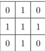
2. We have tested many morphological operators, in which the opening operation g(x) = (f s)⊕s, where g(x) is the output and f is the input image, with a structuring element s of size 3 x 3 (see table 1). In this paper, we have used a small structuring element to capture small tumoral regions and to remove them later using an opening operator. Opening operator uses erosion g(x) =f s, then
dilation g(x) = f ⊕s in succession, where we noticed that this operator improves the results of the 515
first post-processing (i.e., Post-processing 1). We refer to this Post-processing as Post-processing 2.
We have observed that the application of post-processing 1 + post-processing 2 to the output of the
CNNs architectures provides a better segmentation result than the application of a single type of these
0 1 0
1 1 1
0 1 0
Table 1: The used structuring element
4. Experimental results
520
This section presents the results of our experiments and some discussions. Our brain tumor segmentation
method is evaluated using BRATS dataset 2018 which has real patient data with Glioblastomas brain
tumors (both high- and low-grade). Each patient has 4 types of MRI images, firstly we apply a
Pre-processing step (see section 3.1) to these 4 types of MRI images to reduce some noises and to obtain
image Patches with a high quality and resolution. Then we extract Overlapping Patches (see section 3.2) 525
from all these types of MRI images to train the CNNs architectures. The last step is Post-processing (see section 3.5), where we apply to the segmentation results of CNNs architectures (i.e., SparseMultiOCM, InputSparseMultiOCM, DenseMultiOCM) two operations: the first one is the global threshold, and the
second one is the morphological opening operator. Finally, we explain the libraries and frameworks that
are used in our work. Then we evaluate our CNNs architectures with a set of metrics that are used in the 530
state-of-the-art such as Dice score, Sensitivity (Recall), Specificity, and Hausdorff Distance.
4.1. Dataset
We have evaluated our experiments on real patient’s data, in which we have used BRATS 2018 dataset.
The training set has 210 patient’s brain with high-grade (HGG) and 75 patient’s brain with low-grade (LGG).
Each patient’s brain image comes with 4 MRI sequences (i.e., T1, T1c, T2, FLAIR) and the ground truth 535
of 4 segmentation labels which are obtained manually by radiologists experts: Healthy tissue, Necrotic and
Non-Enhancing tumor, Peritumoral Edema, Enhancing core. BRATS 2018 validation set contains 66 images
of patients with an unknown grade, i.e., the validation set does not have the ground truth labels.
4.2. Implementation
To implement our CNNs architectures, we have used Keras which is a high-level open source Deep Learn-540
ing library, and Theano (Al-Rfou et al.,2016) as a Back-end, where Theano exploits GPUs to optimize Deep
Learning architectures (i.e. to minimize the error). In this work, for computing and comparing the inference
time, we used Python environment on Windows 64 bits, Intel Xeon processor CPU @ 3.30 GHz with 8 GB DDR4 RAM, and Nvidia Quadro GPU K2000 with 2 GB GDDR5 memory.
We have tested many techniques for weights initialization: ”Glorot Uniform” (Glorot and Bengio, 2010), 545
”he normal” (He et al., 2015) where he normal initialization provides a fast convergence toward the global
minimum compared to Glorot Uniform, also in this work (He et al., 2016) they found that he normal ini-tialization gives the best results.
The choice of the optimizer plays a very important role in the learning phase, thus, to obtain the best
optimizer for our CNN architectures, we have tested ADAM and RMSProp, Adagrad and SGD optimizers 550
with mini-batch size from 1 to 120, where SGD provides the best results with mini-batch size equals to 8.
The initial learning rate (LR) wasLR0 = 0.001, then it is deceased by theequation 10:
LRi = 10−3×0.99LRi−1 (10)
Where LRi (i ∈ N+) is the new learning rate, LRi−1 is the learning rate of the last epoch, 0.99 is a decreasing factor.
To avoid the Overfitting problem, we have used two methods: (1) BRATS dataset has only 285 MRI images 555
with both high- and low-grade, this number of training data is small to train a Deep Learning model on a
multi-classification problem. Thus, we have used a large number of Overlapping Patches (30.660 Patches)
that provide a better balance of training data among the four classes (i.e. 4 sub-regions) of Glioblastomas
tumors. In addition, the Overlapping Patches technique provides a data augmentation (Hashemi et al.,2019)
to the original BRATS dataset. (2) Theoretically, the error on the training and testing sets decreases after 560
many epochs, but in practice, the error on the testing set at a certain point will start to increase again.
Thus, at this point which is the minimum, the training will be stopped, this method called early stopping.
All our variants of CNNs architectures are trained from scratch using a large number of MRI image Patches
(i.e. 64 ×64×4) equals to 30.660 Patches. Where after many experiments (e.g. 80/20, 60/40), we found that splitting dataset into 70% for training (i.e. first phase) 30% testing (i.e. second phase) is the best 565
distribution, then in the validation phase (i.e. third phase), we have used BRATS 2018 validation set which
contains 66 MRI images of patients with unknown grade. For the evaluation of our CNNs architectures on
the validation dataset, we have used an online evaluation system 2. In addition, our CNNs architectures
trained using MRI images Patches, but these architectures could segment the 3D MRI volume slice-by-slice.
4.3. Evaluation metrics 570
To evaluate the performance of our CNNs architectures, we used BRATS online evaluation system, where
we upload the segmentation results and the system provides the quantitative evaluations contain Dice score,
Sensitivity, Specificity, and Hausdorff distance. For each one of these metrics we have three sub-metrics:
Complete (i.e. Necrotic and Non-Enhancing tumor, Peritumoral Edema, Enhancing tumor), Core (i.e.
Necrotic and Non-Enhancing tumor, Enhancing tumor), Enhancing (i.e. Enhancing tumor). The evaluation 575
metrics are calculated as follows: Dice (P,T) = |P1∧T1| (|P1|+|T1|)/2, Sensitivity (P,T) = |P1∧T1| |T1| , Specificity (P,T) = |P0∧T0| |T0| ,
Hausdorff (P,T) =max{ sup p∈∂P1 inf t∈∂T1 d(p , t), sup t∈∂T1 inf p∈∂P1 d(t , p)}
Where ∧is the logical AND operator, P is the model predictions and T is the ground truth labels. T1 andT0 represent the true lesion region and the remaining normal region respectively. P1 and P0 represent 580
the predicted lesion region and the predicted to be normal respectively. (|.|) is the number of pixels. MRI image is a 3D space (i.e. a set of points inR3): height, width and depth (i.e. a set of slices), each point on
the image is a voxel, and a set of voxels represent a volume. To compute the Hausdorff distance, first we
differentiate the voxels of each class (i.e. creating a map) then we save only the voxels that belong to the
borders of each class, these voxels represent a surface (Voronoi surface). ’p’ and ’t’ are two points on the 585
surface∂P1and∂T1 respectively, and d(p,t), d(t,p) are the shortest least-squares distance between point ’p’ and ’t’ and vice versa for d(t,p). Finally, instead of calculating the maximum distance, we compute only 95%
of the surface distance between each point from the first surface (i.e. the true lesion region) and the other
surface (i.e. the predicted lesion region). This fractional distance is a robust version of Hausdorff because
the existence of outliers can have a considerable impact on the last one (i.e. Hausdorff), also, it is proven 590
that it gives better results than the maximum distance (Menze et al., 2015).
4.4. Results
In this section, we evaluate our CNNs architectures on a public BRATS 2018 dataset. We measure the
segmentation results using four evaluation metrics (see section 4.3), as well as, using the training and the
inference time then we compare our results with the state-of-the-art methods. 595
4.4.1. The effect of class-weighting on the CNNs architectures
Table 2 shows different experiments that are used to train our CNNs architectures where each line
represents a different experiment, also all these experiments are totally independent. We have put our
CNNs architectures under a series of different tests and scenarios: (1) with/without class-weighting, (2)
with/without Bias, with/without regularization techniques such as (3) Instance normalization, (4) Dropout 600
(with different rates), (5) L2 regularization (with different rates), (6) with/without Nestrov Momentum but
these regularization techniques did not improve a lot the segmentation results. In addition, we used Dice
score as a metric to evaluate the CNNs architectures, because this metric represents a trade-off between
sensitivity (recall) and precision and because it’s used in the state-of-the-art BRATS-MICCAI challenges. To demonstrate the performance of Overlapping Patches against Adjacent Patches, we tried different exper-605
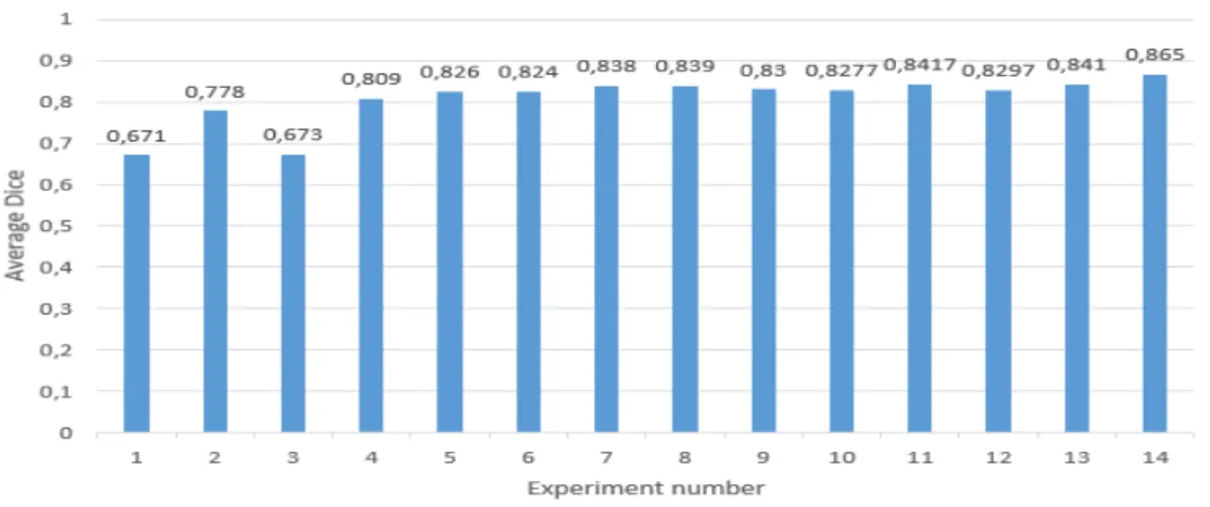
Figure 7: The effect of class-weighting on the CNNs performance. Horizontal axis represents the experiment number in the
table 2(i.e., No.). The vertical axis represents the average Dice score of each experiment (Table 2column 10).
iments where the initial state (i.e. initial parameters) is the same for both types of Patches:
Average Dice= 1 N
X
i Dicei
= Complete+Core+Enhancing 3
(11)
Where N is the number of Dice score sub-metrics (i.e., N=3).
Table 2: the parameters and the results of different and independent experiments of the class-weighting technique. Healthy, Necrotic and Non-Enhancing tumor (NCR/NET), Peritumoral Edema (Edema), Enhancing tumor represent the different Glioblastomas tumor sub-regions, in which we assigned a percentage of contribution for each class. Moreover, for each experiment we show the Dice score of 10 MRI images from BRATS 2018. The last experiment (No = 14) has the best parameters for our proposed CNNs architectures. Fields with (/) mean we did not apply class-weighting technique.
No. Patch type Class-Weights Dice score Average Dice Healthy NCR/NET Edema Enhancing tumor Complete Core Enhancing
1 Adjacent / / / / 0.760 0.595 0.659 0.671 2 Overlap / / / / 0,902 0,8 0,631 0,778 3 Adjacent 0.3 0.2 0.2 0.3 0.772 0.593 0.655 0.673 4 Overlap 0,3 0,2 0,2 0,3 0,899 0,793 0,736 0,809 5 Overlap 0,3 0,15 0,3 0,25 0,909 0,816 0,752 0,826 6 Overlap 0,3 0,12 0,33 0,25 0,901 0,826 0,745 0,824 7 Overlap 0,3 0,1 0,38 0,22 0,906 0,828 0,779 0,838 8 Overlap 0,3 0,06 0,425 0,215 0,912 0,83 0,775 0,839 9 Overlap 0,29 0,05 0,448 0,212 0,903 0,837 0,7505 0,830 10 Overlap 0,29 0,1 0,4 0,21 0,908 0,828 0,747 0,8277 11 Overlap 0,28 0,08 0,43 0,21 0,91 0,838 0,777 0,8417 12 Overlap 0,27 0,08 0,44 0,21 0,905 0,826 0,758 0,8297 13 Overlap 0,27 0,1 0,43 0,2 0,906 0,842 0,775 0,841 14 Overlap 0,28 0,08 0,43 0,21 0,916 0,866 0,812 0,865
1. First: we used Adjacent Patches (i.e.,table 2, first row), and Overlapping Patches (i.e. table 2, second
row) without any class-weighting or regularization techniques and as it is shown in thetable 2andfigure 7, the first experiment with Adjacent Patches achieved on average (see equation 11) 0.671. However, in 610
the second experiment with Overlapping Patches, the CNNs architectures achieved on average 0.778,
which is remarkable that the difference between both experiments is 10.7%.
2. Second: we used Adjacent Patches (i.e.,table 2, third row) and Overlapping Patches (i.e.,table 2, fourth
row), we used also the same mis-classification costs [0.3, 0.2, 0.2, 0.3] for both types of Patches. We
have achieved with Adjacent Patches on average (see equation 11) 0.673. However, with Overlapping 615
Patches, the CNNs architectures achieved on average 0.809, the difference between both experiments
is 13.6%.
In summary, training CNNs architectures with Overlapping Patches always provide a good
segmenta-tion result compared to using adjacent Patches, where we have reported representative results (see table 2)
among all the results. Thus, these experiments demonstrate the effectiveness and the efficiency of Over-620
lapping Patches for training CNNs architectures. Moreover, after trying all these experiments with
dif-ferent configurations to improve the segmentation results of CNNs architectures, we found that the last
experiment (see table 2, experiment No=14) provides the best mis-classification costs (The class-weight of
Healthy tissue=0.28, the class-weight of Necrotic and Non-Enhancing tumor= 0.08, the class-weight of
Per-itumoral Edema= 0.43, the class-weight of Enhanced tumor= 0.21). Furthermore, we note any adjustment 625
of class-weights doesn’t improve the segmentation results. The average Dice score (see equation 11) of each experiment are shownin figure 7.
4.4.2. Segmentation results
In this section, we present the quantitative evaluation on BRATS 2018 validation dataset. First, we
evaluate the segmentation results of each CNNs architecture with and without processing 1 and Post-630
processing 2. Then, we compare these 3 CNNs architectures with the state-of-the-art methods on four evaluation metrics (see section 4.3), and on the training and the inference time in addition to the number of
parameters as a metric.
4.4.2.1 Comparison of CNNs architectures with and without post-processing
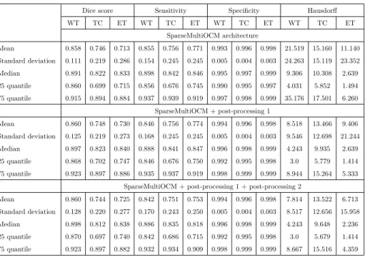
Table 3,table 4,table 5: show the mean score, standard deviation, median, 25 and 75 quantiles for the four 635
metrics: Dice, Sensitivity, Specificity, and Hausdorff distance. It can be observed that our Deep Learning architectures in these 3 tables achieved high results, in which the Mean Dice scores for the 3 architectures on
BRATS validation set are: 0.86, 0.74, 0.74 for whole tumor, tumor core, enhancing tumor respectively. Also,