Linking individual-tree and whole-stand models for forest growth and yield prediction

R E S E A R C H A R T I C L E

Open Access

Linking individual-tree and whole-stand models

for forest growth and yield prediction

Quang V Cao

Abstract

Background:Different types of growth and yield models provide essential information for making informed decisions on how to manage forests. Whole-stand models often provide well-behaved outputs at the stand level, but lack information on stand structures. Detailed information from individual-tree models and size-class models typically suffers from accumulation of errors. The disaggregation method, in assuming that predictions from a whole-stand model are reliable, partitions these outputs to individual trees. On the other hand, the combination method seeks to improve stand-level predictions from both whole-stand and individual-tree models by combining them.

Methods:Data from 100 plots randomly selected from the Southwide Seed Source Study of loblolly pine (Pinus taedaL.) were used to evaluate the unadjusted individual-tree model against the disaggregation and combination methods.

Results:Compared to the whole-stand model, the combination method did not show improvements in predicting stand attributes in this study. The combination method also did not perform as well as the disaggregation method in tree-level predictions. The disaggregation method provided the best predictions of tree- and stand-level survival and growth.

Conclusions:The disaggregation approach provides a link between individual-tree models and whole-stand models, and should be considered as a better alternative to the unadjusted tree model.

Keywords:Disaggregation; Combination method; Loblolly pine;Pinus taeda

Background

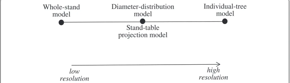
Information provided by growth and yield models is essential for forest managers to make informed decisions on how to manage their forests. Munro (1974) classified growth and yield models into whole-stand models and in-dividual tree models. He further separated inin-dividual-tree models into distance-independent and distance-dependent models. The whole-stand models (low resolution) and individual-tree models (high resolution) represent two ex-tremes. In the middle are medium-resolution models such as diameter-distribution models and stand-table projection models, which provide information for each diameter class (Figure 1).

Each type of model has its own benefits and draw-backs. Whole-stand models often provide well-behaved

outputs at the stand level, but these outputs lack informa-tion on stand structures. Detailed informainforma-tion from individual-tree models and size-class models, on the other hand, typically results in stand-level outputs that are not as accurate or precise because they suffer from accumula-tion of errors (Garcia 2001, Qin and Cao 2006).

Daniels and Burkhart (1988) attempted to link differ-ent types of growth and yield models by developing a framework for an integrated system in which models of different resolutions are related in a unified mathemat-ical structure. The functions used in these models can therefore be considered invariant at different levels of dimensionality.

Zhang et al. (1997) used the multi-response parameter estimation developed by Bates and Watts (1987, 1988) to constrain an individual-tree model by optimizing for both tree and diameter-class levels. This approach was later modified by Cao (2006) to produce a constrained Correspondence:[email protected]

School of Renewable Natural Resources, Louisiana State University Agricultural Center, Baton Rouge, LA 70803, USA

tree model that was optimized for both tree and stand levels.

Disaggregation method is a method that has been used by many researchers for linking an individual-tree model and a whole-stand model (Ritchie and Hann 1997). In this method, outputs from the individual-tree model are adjusted such that the resulting stand summary matches prediction from a whole-stand model.

The disaggregation method above assumes that outputs from whole-stand models are more reliable than those from individual-tree models. Yue et al. (2008) found that stand-level outputs from whole-stand and individual-tree models could be combined to improve predictions. The weighted average approach was extended by Zhang et al. (2010) to include stand-level outputs from a diameter dis-tribution model.

In this paper, the disaggregation method and com-bination method were evaluated against the unadjusted individual-tree model by use of data from unthinned loblolly pine (Pinus taedaL.) plantations.

Review of methods for linking individual-tree models and whole-stand models

Stand-level summary is obtained by aggregating (or sum-ming) tree-level outputs from individual-tree models. Be-cause this summary is often believed to be not as accurate and precise as direct prediction from a whole-stand model, the individual-tree model can be adjusted such that the resulting stand-level output matches that from a whole-stand model. In other words, output from the whole-stand model is disaggregated to tree level by use of some disaggregating function.

Ritchie and Hann (1997) provided an excellent review on disaggregation methods, classifying the disaggregat-ing functions into additive and proportional. In the additive growth method, the basal area growth of each tree is equal to the average tree basal area growth plus an adjustment based on tree basal area (Harrison and

Daniels 1988) or tree diameter (Dhote 1994). Another cat-egory of disaggregation methods involves proportional allo-cations that can be applied to either growth or yield. In the proportional yield method, predicted tree basal area is adjusted to match predicted stand basal area (Clutter and Allison 1974, Clutter and Jones 1980, Pienaar and Harrison 1988, Nepal and Somers 1992, McTague and Stansfield 1994, 1995). The proportional growth method involves adjusting predicted tree basal area growth to match pre-dicted stand basal area growth (Campbell et al. 1979, Moore et al. 1994), tree volume growth to match stand volume growth (Dahms 1983, Zhang et al. 1993), or tree diameter growth to match stand diameter growth (Leary et al. 1979).

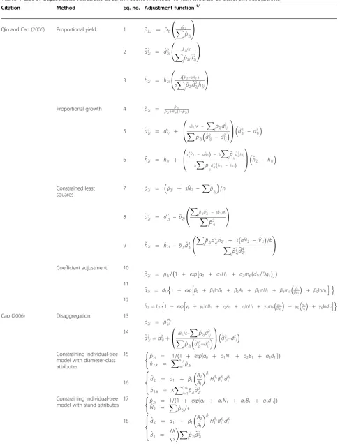
Qin and Cao (2006) evaluated four methods to link an individual-tree model and a whole-stand model by use of disaggregation. In the proportional yield method, the predicted tree survival probability, diameter, and total height were multiplied by adjustment factors (equations 1–3 of Table 1). Tree diameter and height growth were adjusted in the proportional growth method, while tree survival probability was adjusted based on the ratio of dead and alive probabilities (equations 4–6 of Table 1). The constrained least squares method (Matney et al. 1990, Cao and Baldwin 1999) was used to adjust tree attributes (tree survival probability, squared diameter, or total height) by minimizing the sums of squared differences between the predicted and adjusted attributes, subject to the constraints that the aggregations had to match predictions from a whole-stand model (equations 7–8 of Table 1). Finally, in the coefficient adjustment method, adjusting coefficients were added to modify the coefficients of the original individual-tree model to yield stand attributes identical to those produced by the whole-stand model (equations 10–12 of Table 1). The four methods evaluated produced similar results, with the coefficient adjustment selected as the method to disaggregate predicted stand growth among trees in the tree list. The adjusted tree model combined the

low

resolution

Diameter-distribution

model

Individual-tree

model

Stand-table

projection model

high

resolution

Whole-stand

model

Table 1 List of adjustment functions used in recent methods to link models of different resolutions

Citation Method Eq. no. Adjustment function1/

Qin and Cao (2006) Proportional yield 1 ~p2;i ¼ ^p2i s ^ N2

X j^p2j 0 @

1 A

2 ~d2_2i ¼ ^d2_2i s^B2=K X

j^p2jd^

2 2j 0 @ 1 A

3 ~h2i ¼ ^h2i

sðV^2−aN^2Þ

bX j^p2jd^

2 2j^h2j 0

@

1 A

Proportional growth 4 ~p2i ¼ ^p2iþmpp^2ði1−^p2iÞ

5 ~d2_2i ¼ d2_1i þ

s^B2=K −

X j~p2jd

2 1j X

j~p2j d^

2 2j − d

2 1j 0 B @ 1 C

Ad^2_2i − d2_1i

6 ~h2i ¼ h1i þ

sðV^2 − aN^2Þ − b

X j~p2j

~ d2

2jh1j

b X

j~p2j ~ d2

2jðh^2j − h1iÞ 0

B @

1 C

A ^h2i − h1i

Constrained least squares

7 ~p2i ¼ ^p2i þ s^N2 −

X ^ p 2j =n

8 ~d2

2i ¼ ^d22j − ~p2i X

jp~2jd^22j − s^B2=K

X j~p

2 2j 0 @ 1 A

9 ~h2i ¼ ^h2i − p~2i~d22i X

j~p2j~d

2

2jh^2j þ s aN^2 − V^2

=b X

jp~

2 2jd~

4 2j 0 @ 1 A

Coefficient adjustment 10

~

p_2i ¼ p_1i= 1 þ expα0 þ α1H1 þ α2mpðd1i=Dq1Þ

11

~

d2i ¼ d1i 1 þ exp β0 þ β1lnB1 þ β2A1 þ β3lnH1 þ β4md Dqd1i1 þ β5lnh1i

h i

n o

12

~

h2i¼h1i 1 þ expγ0 þ γ1lnB1 þ γ2A1 þ γ3lnH1 þ γ4mh Dqd1i1 þ γ5 h1i

H1 þ γ6lnd1i

h i

n o

Cao (2006) Disaggregation 13

~ p2i ¼ ^p

mp

2i 14

~

d2_2i¼d2_1iþ s

^

B2=K−X_j~p2jd21j X

j~p2j d^

2 2j−d

2 1j 0 B @ 1 C Ad^2_2i−d2_1i

Constraining individual-tree model with diameter-class attributes

15 _^p

2i ¼ 1=ð1 þ exp½α0 þ α1N1 þ α2B1 þ α3d1iÞ

^ n2;k ¼

Xn1;k i¼1^p2i

(

16 d^2i ¼ d1i þ β1

A2

A1

β2

Hβ3

1B β4 1d β5 1 ^ b2;k ¼ K

Xn1;k i¼1p^2i^d

2 2i 8 > < > : Constraining individual-tree model with stand attributes

17 _^p

2i ¼ 1=ð1 þ exp½α0 þ α1N1 þ α2B1 þ α3d1iÞ

^

N2 ¼ X

i^p2i=s (

18 d^2i ¼ d1i þ β1

A2

A1

β2

Hβ3

1Bβ14dβ15

^ B2 ¼

K s X

i^p2id^

best features of whole-stand and individual-tree models. Compared to the unadjusted tree model, the adjusted model performed better in predicting stand attributes in terms of stand density, basal area, and volume, especially for long projection periods. The adjusted model also

provided comparable predictions of tree diameter, height, and survival probability.

Cao (2006) evaluated a disaggregation method against two approaches to constrain an individual-tree model. In the disaggregation method, the predicted tree survival Table 1 List of adjustment functions used in recent methods to link models of different resolutions(Continued)

Yue et al. (2008) Combined estimator 19 ~B2 ¼ w^B2T þ ð1 wÞ^B2S,

wherewis selected to minimize the variance of~B2.

Zhang et al. (2010) Combined estimator 20

~

B2¼w1^B2Tþw2^B2Sþw3^B2D,

wherewkis selected to minimizeXB2−~B2

2

, andX3 kwk¼1.

Cao (2010) 1 21

~ p_2i¼^pm

2i

Tree survival 2 22

~

p2i¼^p2i þ mpp^2ði1 − ^p2iÞ

3 23

~

p_2i ¼ 1=1 þ exp mpα0þα3d1i

4 24

~

p2i ¼ 1=1 þ expα0þα1N1þα2B1þmpd1i

5 25

~

p_2i¼^p_2iþ s

^ N2 −

X jp^2j sN1 −

X j^p2j 0

@

1 Að1−^p_2iÞ

Cao (2010) 1 26

^

d2i ¼ d1i þ mddβ15

Tree diameter growth 2 27

^

d2i ¼ d1i þ β1 AA21 β2

Hβ3

1Bβ14d

md

1

3 28

~

d2_2i ¼ d2_1i þ

s^B2=K−

X j~p2jd

2 1j X

j~p2j d^

2 2j−d21j

0 B @

1 C Ad^2_2i−d2_1i 1/

Notation:

A1= stand age at the beginning of the growth period.

A2= stand age at the end of the growth period.

H1= dominant height at ageA1.

N1= number of trees per ha at ageA1.

^

N2= predicted number of trees per ha at ageA2. B1= stand basal area at ageA1.

^

B2= predicted stand basal area at ageA2. ^

B2D= predicted stand basal area at ageA2from a diameter distribution model.

^

B2S= predicted stand basal area at ageA2from a whole-stand model.

^

B2T= predicted stand basal area at ageA2from an individual-tree model.

~

B2= combined estimator for stand basal area at ageA2. ^

V2= predicted volume per ha at ageA2,Dq1= quadratic mean diameter at ageA1.

aandb= parameters of the individual tree volume equation,vi ¼ a þ bd2ihi. vi,di, andhi= tree volume, dbh, and total height of treei, respectively. s= plot size in ha.

K=π/40 000 = constant to convert diameter in cm to area in m2.

n= number of trees in the plot.

d1iord1j= dbh of treeiorjat ageA1. ^

d2iord^2j= predicted dbh of treeiorjat the end of the growth period.

~

d2i= adjusted dbh of treeiat the end of the growth period. h1i= total height of treeiat ageA1.

^

h2iorh^2j= predicted total height of treeiorjat the end of the growth period.

~

h2i= adjusted total height of treeiat the end of the growth period. p1i= survival probability of treeiat ageA1.

^

p2ior^p2j= predicted survival probability of treeiorjat the end of the growth period.

~

p2ior~p2j= adjusted survival probability of treeiorjat the end of the growth period.

α0…α3= parameters of the tree survival equation. β0…β5= parameters of the tree diameter growth equation. γ0…γ6= parameters of the tree height growth equation.

n1,k= number of trees of thekthdiameter class at ageA1. ^

n2;k= predicted number of trees of thekthdiameter class at ageA2.

^

probability was adjusted with a simple power function, in which the power was iteratively solved such that the adjusted survival probability summed up to the pre-dicted stand density (equation 13 of Table 1). The pro-portional growth formula was used in adjusting diameter growth (equation 14 of Table 1). The individual-tree model was constrained by diameter-class attributes (equations 15–16 of Table 1) by use of the multi-response parameter estimation method (Zhang et al. 1997, Bates and Watts 1987, 1988). Also included in the evaluation was a similar approach to constrain the individual-tree model by stand attributes (equations 17–18 of Table 1). Cao (2006) found that while the two constrained models performed slightly better than the unconstrained tree model in predicting tree and stand attributes, the disaggregation method provided the best predictions of tree- and stand-level survival and growth.

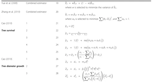
Cao (2010) listed different disaggregation methods for predicting tree survival and diameter growth. These in-clude five disaggregation methods for adjusting tree sur-vival probability (equations 21–25 of Table 1) and three methods for diameter growth adjustment (equations 26–28 of Table 1). His results showed that the different methods produced similar results. Cao (2010) also found that use of observed rather than predicted stand attri-butes for disaggregation led to improved predictions for tree survival and diameter growth, i.e. the quality of the tree-level predictions in disaggregation depended on the reliability of the stand predictions.

Yue et al. (2008) used the method introduced by Bates and Granger (1969) and Newbold and Granger (1974) to combine stand-level outputs from whole-stand and individual-tree models. The combined estimator is a weighted average of outputs from both models (equation 19 of Table 1). The optimum weights were selected to minimize the the variance of the combined estimator. Zhang et al. (2010) extended this approach to also in-clude stand-level outputs from a diameter distribution model (equation 20 of Table 1). The least-squares esti-mate of the weights was computed according to Tang (1992, 1994).

Methods

Stand- and tree-level growth models developed by Cao (2006) were used in this study. The whole-stand model consisted of equations for predicting stand density in terms of number of trees and basal area per hectare as follows:

^

N2;i¼N1;i=½1 þ exp

16:3197–42:4204 RS1;i –0:7466 H1;i

–0:0269N1;i=A1þ50:2622=A1Þ;

ð1Þ

^

B2;i¼B1;i=1 þ exp–3:3259–0:7800 B1;i=A1þ41:0393=A1

ð2Þ where:

N1,i= number of trees per ha in plotiat ageA1,

^

N2;i = predicted number of trees per ha in plot i at

ageA2,

H1,i= average dominant and codominant height (m) of

plotiat ageA1,

RS1,i= (10,000/N1,i)0.5/ H1,i= relative spacing of ploti

at ageA1,

B1,i= stand basal area (m2/ha) of plotiat ageA1, and

^

B2;i = predicted stand basal area (m2/ha) of plot i at

ageA2.

The individual-tree model included equations for pre-dicting tree survival probability and diameter growth as follows:

^

pij¼ 1þexp 1:3586−0:0010N1;iþ0:1042B1;i−0:2902d1;ij

−1

ð3Þ

^

d2;ij¼d1;ijþ0:7168 A2

A1

2:0192

H1;i−1:0111B1;i−0:3166d1;ij1:5117

ð4Þ

where:

^

pij = predicted probability that treejin ploti is alive

at ageA2, given that it was alive at ageA1,

d1,ij= diameters (cm) of treejin plotiat ageA1, and

^

d2;ij = predicted diameters (cm) of tree j in plot i at

ageA2.

Data

Equations (1, 2, 3 and 4) above were derived from 100 plots from loblolly pine (Pinus taeda L.) plantations in the Southwide Seed Source Study, which include 15 seed sources planted at 13 locations across 10 southern states (Wells and Wakeley 1966).

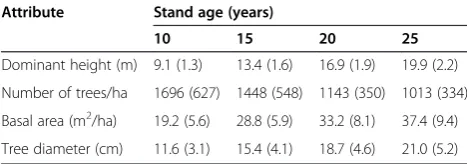
Data used in this study were from another 100 plots, also randomly selected from the Southwide Seed Source Study. Each 0.0164 ha plot consisted of 49 trees, planted at a 1.8 m × 1.8 m spacing. Tree diameters and survival were recorded at ages 10, 15, 20, and 25 years, resulting in a total of 300 growth periods (Table 2).

Methods evaluated

In addition to the individual-tree model (equations 3 and 4), the disaggregation and combination methods were evaluated in this study.

Disaggregation method

The tree survival probability (p^ij) predicted from

~

pij¼^pija ð5Þ

whereα is the adjustment coefficient used to match the sum of adjusted tree survival probabilities (~pij) to predic-tions from the stand survival model (equation1).

From equation (4), the projected tree diameter (d^2;ij)

was adjusted (Cao 2010) so that the resulting stand basal area matches the prediction from the whole-stand model (equation 2):

~

d22;ij¼d21;ijþβ d^22;ij−d21;ij

ð6Þ

where:

β¼ sBb2;i=K−

X

~ p_ijd21;ij

X

~

pij d^22;ij−d21;ij

h i, and:

K=π/40 000.

Combination method

The combined estimator of stand survival was the weighted average of stand-level predictions from the whole-stand model (equation 1) and the individual-tree model (equation 3). The weights were computed according to a method described by Tang (1992, 1994) and applied by Zhang et al. (2010). A similar procedure was applied to compute the combined estimator for stand basal area.

Predictions from the individual-tree model were then adjusted from the combined estimators for stand survival and basal area, using the disaggregation method described earlier.

Evaluation criteria

The performance of the unadjusted, disaggregation, and combination methods was evaluated at both stand and tree levels, based on the following statistics.

Mean difference:

MD ¼Xðyi−^yiÞ=n ð7Þ

Mean absolute difference:

MAD¼Xjyi−^yij=n ð8Þ

FI¼Xðyi−^yiÞ

2₌

yi−y

ð Þ2 _ð

9Þ

Log-likelihood:

−2lnð Þ ¼L −2 Xpilnð Þ þpi X

1−pi

ð Þln 1ð −piÞ

h i

ð10Þ

where:

yiand^yi= observed and predicted values at the end of

the growth period of stand variables (stand survival and basal area) or tree variables (tree diameter and survival probability),

y = average ofyi,

n= number of observations, and

pi= predicted survival probability of treei.

Results and discussion

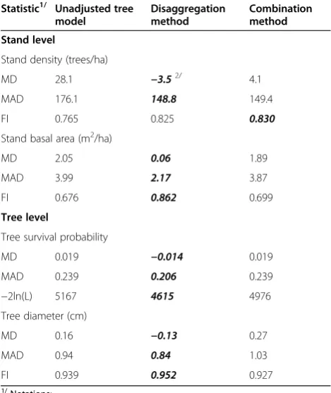
Table 3 shows that the whole-stand model (disaggrega-tion method) produced the best MD and MAD values for stand density while the combination method yielded the best FI value. For stand basal area, all of the best evaluation statistics came from the whole-stand model (Table 3). At tree level, the disaggregation method returned the best evaluation statistics for both tree sur-vival probability and tree diameter (Table 3).

Disaggregation method

From Table 3, it is clear that the whole-stand model was more accurate (lower MD) and precise (lower MAD and higher FI) in predicting stand density and basal area than the individual-tree model. The differences were substantial. Compared to the individual-tree model, the whole-stand model decreased MD by 88 and 97%, de-creased MAD by 15 and 46%, and inde-creased FI by 8 and 28% for stand density and stand basal area, respectively. Predicted stand attributes from the tree-level model were not as reliable because they were obtained through summation of individual-tree predictions, resulting in accumulation of error.

Qin and Cao (2006) showed that a tree-level model, after being adjusted from observed stand attributes through disaggregation, outperformed the unadjusted tree model. They inferred that the performance of disag-gregation models depended largely on how close the stand predictions were to the observed values. The whole-stand model seemed a good candidate in this case, yielding FI values of 0.825 and 0.862 in predicting stand density and basal area, respectively. The tree-level statistics support this hypothesis: the disaggregation model reduced MD by 26 and 19%, and MAD by 14 and 11% for tree survival probability and tree diameter, re-spectively, as compared to the unadjusted tree model. It Table 2 Means (and standard deviations) of stand and

tree attributes, by age

Attribute Stand age (years)

10 15 20 25

Dominant height (m) 9.1 (1.3) 13.4 (1.6) 16.9 (1.9) 19.9 (2.2)

Number of trees/ha 1696 (627) 1448 (548) 1143 (350) 1013 (334)

Basal area (m2/ha) 19.2 (5.6) 28.8 (5.9) 33.2 (8.1) 37.4 (9.4)

Tree diameter (cm) 11.6 (3.1) 15.4 (4.1) 18.7 (4.6) 21.0 (5.2)

also decreased –2ln(L) for tree survival by 11% and in-crease FI for tree diameter by 1%.

Combination method

In this study, combining stand predictions from the whole-stand and individual-tree models resulted in pre-dictions of stand density and basal area that were better than those from the individual-tree model, but not as good as those from the whole-stand model. Among six evaluation statistics considered, the combination method only edged the whole-stand model in fit index (0.830 versus 0.825), while came in second for the remaining statistics. This was contrary to past reports of superior performance by the combination method (Yue et al. 2008, Zhang et al. 2010). In a study by Zhang et al. (2010), similar fit index values, ranging from 0.9466 to 0.9494, were obtained for predicted stand basal area from three different types of models for the validation data set. In this study, a considerable difference in fit index of stand basal area prediction between the individual-tree model (0.676) and the whole-stand model (0.862) might

result in mediocre performance of the combination method (FI = 0.699 for stand basal area).

The tree survival model that was disaggregated from the combined estimator gave similar evaluation statistics as did the unadjusted tree survival equation (Table 3). On the other hand, the tree diameter model from the combin-ation method performed worse than the unadjusted tree diameter growth equation (Table 3).

Tree-level predictions were disaggregated from the whole-stand model for the disaggregation method and from the combined estimator for the combination method. Based on the data from this study, the disaggregation method was better for predicting both tree survival and diameter in terms of all evaluation statistics.

Conclusions

The disaggregation method involves adjusting outputs from the individual-tree model to match predictions from the whole-stand model. It was shown in previous findings and also in this study that this method provided better predictions of tree survival and diameter growth. Compared to the whole-stand model, the combination method did not show improvements in predicting stand attributes in this study. The combination method also did not perform as well as the disaggregation method in tree-level predictions.

Competing interest

The author declares that he has no competing interests.

Acknowledgement

Funding for this project was provided in part by the McIntire-Stennis funds.

Received: 25 July 2014 Accepted: 4 September 2014

References

Bates DM, Watts DG (1987) A generalized Gauss-Newton procedure for multi-response parameter estimation. SIAM J Sci Stat Comput 8:4–55 Bates DM, Watts DG (1988) Nonlinear regression analysis and its application.

Wiley, New York. 365

Bates JM, Granger CWJ (1969) The combination of forecasts. Oper Res Q 20:451–468 Campbell RG, Ferguson IS, Opie JE (1979) Simulating growth and yield of

mountain ash stands: a deterministic model. Aust For Res 9:189–202 Cao QV (2006) Predictions of individual-tree and whole-stand attributes for

loblolly pine plantations. For Ecol Manage 236:342–347

Cao QV (2010) Adjustments of individual-tree survival and diameter growth equations to match whole-stand attributes. In: Proc of the South Silvic Res Conf USDA For Serv Gen Tech Rep SRS-121, pp 369–373

Cao QV, Baldwin VC, Jr (1999) A new algorithm for stand table projection models. Forest Sci 45:506–511

Clutter JL, Allison BJ (1974) A growth and yield model forPinus radiatain New Zealand. In: Fries J (ed) Growth Models for Tree and Stand Simulation, Res. Note 30. Royal College of Forestry, Stockholm, pp 130–160

Clutter JL, Jones BJ, Jr (1980) Prediction of Growth after Thinning of Old-Field Slash Pine Plantations. USDA For Serv Res Pap SE-217, p 14

Dahms WG (1983) Growth-Simulation Model for Lodgepole Pine in Central Oregon. USDA For Serv Res Pap PNW-302, p 22

Daniels RF, Burkhart HE (1988) An integrated system of forest stand models. For Ecol Manage 23:159–177

Dhote JF (1994) Hypotheses about competition for light and water in even-aged common beech (Fagus silvaticaL). For Ecol Manage 69:219–232

Table 3 Stand-level and tree-level evaluation statistics for three methods

Statistic1/ _{Unadjusted tree}

model

Disaggregation method

Combination method

Stand level

Stand density (trees/ha)

MD 28.1 −3.52/ 4.1

MAD 176.1 148.8 149.4

FI 0.765 0.825 0.830

Stand basal area (m2/ha)

MD 2.05 0.06 1.89

MAD 3.99 2.17 3.87

FI 0.676 0.862 0.699

Tree level

Tree survival probability

MD 0.019 −0.014 0.019

MAD 0.239 0.206 0.239

−2ln(L) 5167 4615 4976

Tree diameter (cm)

MD 0.16 −0.13 0.27

MAD 0.94 0.84 1.03

FI 0.939 0.952 0.927

1/ Notations:

MD =Xðyi−^yiÞ=n; MAD =

X

yi−y^i

j j=n; FI =Xðyi−^yiÞ

2

=ðyi−yÞ

2 ;−2 ln (L) =−2[∑piln(pi) +∑(1−pi)ln(1−pi)], whereyiandy^i= observed and predicted

values at the end of the growth period of stand variables (stand survival and basal area) or tree variables (tree diameter and survival probability);y= average ofyi;n= number of observations, andpi= predicted survival probability of treei.

2/

Garcia O (2001) On bridging the gap between tree-level and stand-level models. In: Rennolls K (ed) Proceedings of IUFRO 4.11 Conference“Forest Biometry, Modelling and Information Science”. University of Greenwich. 25–29 June 2001 http://cms1.gre.ac.uk/conferences/iufro/proceedings/garcia1.pdf Harrison WC, Daniels RF (1988) A new biomathematical model for growth and

yield of loblolly pine plantations. In: Ek AR, Shifley SR, Burk TE (ed) Forest Growth Modeling and Prediction, vol 1. USDA North Central Forest Experiment Station, St. Paul, MN, pp 293–304. USDA For Serv Gen Tech Rep NC-120

Leary RA, Holdaway MR, Hahn JT (1979) Diameter growth allocation rule. In: A generalized forest growth projection system applied to the Lake States region. USDA For Serv Gen Tech Rep NC-49, pp 39–46

Matney TG, Belli KL, Farrar RM, Jr (1990) Parameter-free diameter-distribution recovery. In: Division 4 Proceedings of the IUFRO World Congress Meeting, Montréal, Que., Canada, 5–11 August 1990. Publ. FWS-2-90. School of Forestry and Wildlife Resources, Virginia Polytechnic Institute and State University, Blacksburg, Va, pp 95–107

McTague JP, Stansfield WF (1994) Stand and tree dynamics of uneven-aged ponderosa pine. Forest Sci 40:289–302

McTague JP, Stansfield WF (1995) Stand, species, and tree dynamics of an uneven-aged, mixed conifer forest type. Can J Forest Res 25:803–812 Moore JA, Zhang L, Newberry JD (1994) Effects of intermediate silvicultural

treatments on the distribution of within-stand growth. Can J Forest Res 24:398–404

Munro DD (1974) Forest growth models–a prognosis. In: Fries J (ed) Growth Models for Tree and Stand Simulation, Res. Note 30. Royal College of Forestry, Stockholm, pp 7–21

Nepal SK, Somers GL (1992) A generalized approach to stand table projection. Forest Sci 38:120–133

Newbold P, Granger CWJ (1974) Experience with forecasting univariate time series and the combination of forecasts. J R Stat Soc Ser A 137:131–165 Pienaar LV, Harrison WM (1988) A stand table projection approach to yield

prediction in unthinned even-aged stands. Forest Sci 34:804–808 Qin J, Cao QV (2006) Using disaggregation to link individual-tree and whole-stand

growth models. Can J Forest Res 36:953–960

Ritchie MW, Hann DW (1997) Implications of disaggregation in forest growth and yield modeling. Forest Sci 43:223–233

Tang X (1992) Forecasting Theory with its Applications (in Chinese with English abstract). University of Electronic Science and Technology of China, Chengdu, China. 288

Tang X (1994) Some new results of the efficient frontier of portfolio investment. J UEST China 23:301–305

Wells OO, Wakeley PC (1966) Geographic variation in survival, growth, and fusiform rust infection of planted loblolly pine. Forest Sci Monogr 11:40 Yue CF, Kohnle U, Hein S (2008) Combining tree- and stand-level models: a new

approach to growth prediction. Forest Sci 54:553–566

Zhang L, Moore JA, Newberry JD (1993) Disaggregating stand volume growth to individual trees. Forest Sci 39:295–308

Zhang S, Amateis RL, Burkhart HE (1997) Constraining individual tree diameter increment and survival models for loblolly pine plantations. Forest Sci 43:414–423

Zhang X, Lei Y, Cao QV (2010) Compatibility of stand basal area predictions based on forecast combination. Forest Sci 56:552–557

doi:10.1186/s40663-014-0018-z

Cite this article as:Cao:Linking individual-tree and whole-stand models for forest growth and yield prediction.Forest Ecosystems20141:18.

Submit your manuscript to a

journal and benefi t from:

7 Convenient online submission 7 Rigorous peer review

7 Immediate publication on acceptance 7 Open access: articles freely available online 7 High visibility within the fi eld

7 Retaining the copyright to your article