Transmission Line Fault Location based on Distributed Parameter Line Model

(1)

Vol. 4, Issue 3, March 2015

Transmission Line Fault Location based on

Distributed Parameter Line Model

Ashish N. Kakde

M. Tech Scholar, Dept. of Electrical Engineering, Govt. College of Engineering, Amravati, Maharashtra, India

ABSTRACT:In this article an algorithm for transmission line fault location is discussed. This algorithm is based on Distributed Parameter Line Model which utilizes unsynchronized voltage and current measurements from two ends of the line. Firstly, the algorithm is derived, based on Distributed Parameter line model, then the simulation is carried out in MATLAB to obtain the fault voltages and currents at both ends of a transmission line. Then, with the help of Newton-Raphsonapproach based iterative method simulated data is used for estimating the location of faults (unbalanced and balanced) on line. It is observed that solution is independent of fault resistance and source impedance. Evaluation studies based on MATLAB/SIMULINK Simulation studies have been undertaken to verify the accuracy of the algorithm.

KEYWORDS:distributed parameter line model, fault location, unsynchronized.

I.INTRODUCTION

In Electrical Power Systems, Transmission lines are prone to various faults. It is very necessary that faults occurring at lines must be located accurately so that maintenance crew members arrive at the place and fix the faulty section as soon as possible. As we know physical constraints causes some parts of power transmission lines to be difficult to reach. Hence, validity of the accurate fault location detection under several of power system operating constraints and fault conditions is an important necessity. Normally, quick and exact fault location expedites supply restoration and enhances the supply quality and reliability [1]. When any kind of faults occur in a power system, the first action must be to clear the fault from the system. Once the protection action is taken, the most accurate distance of fault information should be provided to aid the user in locating the fault to remove the cause of the fault. Fault location can be estimated from current and voltages measured from one-end or two-end of the line [2].

Following the fault, the public utility company tries to re-establish the power as fast as possible. Rapid restoration of service reduces user’s grievances, time of breakdown, loss of taxation and expenses of crew repair. All of these factors are increasingly important to the utilities facing challenges in today’s market. To aid in rapid and efficient service restoration, algorithms have been developed to provide an estimate of the fault location.In this paper for the enhancement of the computational efficiency, instead of EMTP software, MATLAB software is used.Further, by using these voltages and currents phasor values,iterative method is used for calculating an accurate fault location.It is observed that Newton-Raphson based iterative method involving an unsynchronized algorithm based on distributed parameter model gives better and precise results in locating the faults at transmission line.

II.RELATED WORK

(2)

III.VARIOUS FAULT LOCATION ALGORITHMS

Recognizing the importance as well as the challenges in fault location, a number of researchers have worked in this area and developed a valuable set of algorithms. Based on the available data, one-terminal [4], two-terminal [5], or multi terminal algorithms [6] have been proposed in the past. Most algorithms are based on an principle of impedance, which make use of the fundamental frequency currents and voltages.

A one-terminal algorithm uses data (local voltages and currents) from just one end of the transmission line. The accuracy of this type of algorithm is normally adversely affected by fault resistance, and a compensation technique is needed to alleviate this effect. One-end impedance-based fault location algorithms estimate a distance to fault with the use of voltages and currents acquired at a particular end of the line. Such a technique is simple and does not require communication channel with the distant end. Hence, it is appealing and is vividly incorporated into the microprocessor-based protective relays. However, it is subject to several errors, such as the effect of reactance, shunt capacitance of line, and the fault resistance value. Two terminal algorithms processes signals from both the ends of transmission line. Hence large amount of information can be utilized. Performance of the two-end algorithms is generally superior in comparison to the one-end approaches.

The second class of algorithms are based on traveling wavein which methods time-tags the arrival of the first high-frequency pulse due to a fault, at each end of the line. From knowledge of the surge impedance of the line, the length of the line and the difference between the time of arrival of the first pulse at each line end, the fault location can be determined. Some papers proposed the use of wavelets [7] to decompose the sampled voltage and current data to determine the time of arrival of the high frequency fault pulse. Some papers propose fault location techniques based on artificial neural networks [8]. Online fault detection techniques employing GPS make use of synchronised sampling of data. But malfunctioning in this may lead to inaccurate fault location. Hence unsynchronised sampling of two end data is considered to be better method of fault location [9, 10, 11].

This paper discusses a fault location algorithm utilizing the fundamental frequency phasors of voltages and currents from two ends of the line depending on line model [12, 13, 14, 15] consisting of Distributed Parameters which fully considers the shunt capacitance and distributed parameter effects. The developed solution is independent of fault impedance and source impedance, and does not require data synchronization between measurements at two ends of the line. Following sections presents the proposed method with results and discussions.

IV.FAULT LOCATION METHOD

Consider the line between terminals P and Q, as shown in Figure 1, where EP and EQ represent the Thevenin equivalent sources.

Fig.1.Transmission Line considered for analysis

Fig 2 depicts the mode 1 equivalent



circuit of the line during the fault [11]. R indicates the fault point.

E

P

E

Q

(3)

Fig.2. Positive sequence network of the system during the fault Based on fig 2, we obtain

1 1 1 1 1 1

2 2

pr qr j

p pr p p q qr q q

Y Y

V Z _I V __V Z _I V __e

     ₍₁₎

Where,Zpr_and Zqr_{equivalent series impedance of the line segment PR and QR.}

Y

pr_and

Y

qr_{are equivalent shunt}

admittance of the line segment PR and QR.Vp1_andIp1_{mode 1 voltage and current during the fault at P.}Vq1_andIq1_mode

1 voltage and current during the fault at Q.is the synchronizing angle. The equivalent transmission line parameters depending on the distributed model are as follows:

1 1 c z Z y  (2) 1 1 z y

 ₍₃₎

 

1

sinh

pr c Z Z l

(4)



1



sinh

qr c

Z Z _ l l _

(5) 1 2 tanh 2 pr c l Y Z     _ _

 ₍₆₎



1



2 tanh 2 qr c l l Y Z      _ _

 ₍₇₎

Where

c

Z _{Characteristic impedance of the line;}



_{Propagation constant of the line;}

l

Length of the line in km or mile;

1

l

Fault distance from P to R in km or mile Substituting Equations (2) to (7) in (1) results in













1

1 1 1 1 1

1

1 1 1

1

( ) sinh tanh

2 1

sinh tanh 0

2

j

p c p p q

c

j

c q q

c

l

f x V Z l I V V e

Z

l l

Z l l I V e

Z            _  _ __             _   _   

  ₍₈₎

2 pr Y 2 pr Y 2 qr Y 2 qr Y pr

Z Zqr Iq1

1

p

I

1

p

V Vq1

1 f

I

1 f V

(4)

where



1



T

x



l



, T represent vector transpose operator. There are two unknown variables in Equation (8), solution of which is presented as follows.Equation (8) is a complex equation and can be separated into two real equations corresponding to its real and imaginary part as

 



 



1 Re 0

f x  al f x  ₍₉₎

 



 



2 Im 0

f x  ag f x  ₍₁₀₎

where Real(.) and Imag(.) yield the real and imaginary part of its arguments, respectively. It follows that

 

1

1 1

Re

f x f x al l l     _ _  _  _ (11)

 

1 Re

f x f x al       _ _  _  _ (12)

 

2 1 1 Im

f x f x ag l l     _ _  _  _ (13)

 

2 Im

f x f x

ag

 

  

 _ _

 _  _₍₁₄₎

Now define

 

1 1 1 2 2 1

f x f x l

J x

f x f x l        _ _    _ _        

 ₍₁₅₎

 

1

 

2

 

T

F x  _f x f x _

(16)

Then the unknown variable

x

can be obtained using the Newton-Raphson approach iteratively as follows:

 

1 1

k k k

x_ x J F x

(17) Where

1

k

x

_



Solution of

x

after

k

th_iteration;

k



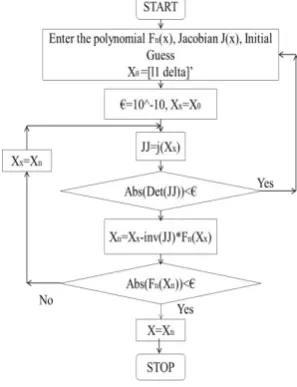
_{Iteration number starting from one.}

Fig 3 below shows the Newton-Raphson approach with the help of flowchart.

(5)

4.1 EVALUATION STUDIES

To get the voltage and current measurement data at both ends of a transmission line during the fault, a simulation using the SIMULINK has been carried out for a fault at 150km. A500kV, 320km long transmission-line is considered for the simulation purpose. The fault distance is assumed to be at a distance 150km from terminal P.

In order to get precise fault location per-unit system is utilized with a voltage base of 500kV and an apparent power base of 100 MVA. The voltage and current phasor values from both source side P and Q are obtained from SIMULINK model for line-to-ground fault (L-G).The accuracy of above algorithm is measured by the percentage error calculated as

(18)

The data of voltage and current phasors obtained from SIMULINK is fed to a MATLAB based programming in order to locate the transmission line fault location [16]. Further in order to get positive sequence values (mode 1 components) a conversion is made from unsymmetrical to symmetrical one. Out of six parameters (V_p₁,I_p₁,V_q₁, I_q₁,Z_C,



) value of Z_C

and



is calculated using equation (2) and equation (3) for a particular transmission line module considered in SIMULINK.

Fig. 4. Model of Transmission line connected with two end sources.

The voltage and current waveforms at terminal P obtained from SIMULINK model during L-G fault are shown in fig 6. Similarly, the voltage and current waveforms at terminal Q are shown in fig 7. Prior to fault the voltage and current waveforms are depicted in fig 5.

Fig.5. Voltage and Current prior to the Fault

(6)

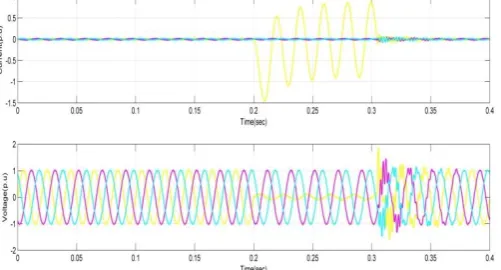
Fig.6. Voltage and Current at Bus P with fault at 150 km

Fig. 6 shows the waveforms of current and voltages after occurrence of fault. The current has increased to higher value of particular faulty phase and voltage has fallen below the rated value.

Fig.7. Voltage and Current at Bus Q with fault at 150km

V.RESULTS AND DISCUSSION

For the Newton-Raphson based iterative method, starting value for



is chosen to be zero in all the cases.

Fig. 8. MATLAB Code for fault location

(7)

By giving the intial input arguments to the program it evaluates the fault location and synchronising angle. Iteration counter limit is set at 30.

TABLEI.DETERMINATION OF FAULT LOCATION WITH USE OF POSITIVE SEQUENCE QUANTITIES

Fault Types Actual Location (km)

Estimated Location

(km)

Error (%)

LG 50 47.91 0.006 100 97.60 0.075 150 140.8 0.028

LL 50 48.85 0.003 100 99.14 0.002 150 142.05 0.024

LLG 50 51.07 -0.003 100 98.01 0.006 150 145.01 0.015

LLL 50 49.01 0.003 100 98.21 0.005 150 147.20 0.008

As can be seen from the Table, for various fault locations, estimated location obtained from the algorithm seems to be nearer to actual location with a difference of few kilometres in some cases. Accuracy can be increased by utilizing exact data of voltages and currents obtained during the fault.

V. CONCLUSION

The discussed algorithm is tested for various fault resistance (0 ohm, 5 ohm, 10 ohm etc.) for voltages and current data obtained from two end of transmission line. Again various types of faults are taken under study in order to get check the accuracy and sensitivity of an algorithm. It is observed that the error calculated using formula lies well below 1%.

REFERENCES

[1] H. Al-Mohammed and M. A. Abido, “Fault Location Based on Synchronized Measurements:A Comprehensive Survey”, Hindawi Publishing Corporation, The Scientific World Journal, Volume 2014, Article ID 845307, 10 pages

[2] Alkım Çapar and Ayşen Basa Arsoy, “Evaluating Accuracy of Fault Location Algorithms Based on Terminal Current and Voltage Data”, International Journal of Electronics and Electrical Engineering, Vol. 3, No. 3, June 2015.

[3] Abdolhamid Rahideh, Mohsen Gitizadeh and Sirus Mohammadi, “ A Fault Location Technique for Transmission Lines Using Phasor Measurements”, International Journal of Engineering and Advanced Technology (IJEAT) ISSN: 2249 – 8958, Volume-3, Issue-1, October 2013. [4] J. Izykowski, E. Rosolowski and M. Mohan Saha, “Locating faults in parallel transmission lines under availability of complete measurements at one end”, IEE Proceeding.-Generation Transmission Distribution, Vol. 151, No. 2, March 2004.

[5] Damir Novosel, David G. Hart, Eric Udren and Jim Garitty, “Unsynchronized Two-Terminal Fault Location Estimation”, IEEE Transactions on Power Delivery, Vol. 11, No. 1, January 1996.

[6] Adly A. Girgis, David G. Hart and William L. Peterson, “A New Fault Location Technique For Two- And Three-Terminal Lines”,IEEE Transactions on Power Delivery, Vol. 7 No.1, January 1992.

[7] Sunusi Sani Adamu,Sada Iliya, “Fault Location and Distance Estimation on Power Transmission Lines Using Discrete Wavelet Transform”,International Journal of Advances in Engineering & Technology,Vol. 1, Issue 5, pp. 69-76,Nov 2011.

[8] Sanjay Kumar K,Shivakumara Swamy.R,V. Venkatesh, “Artificial Neural Network based Method for Location and Classifications of Faults on a Transmission Lines”,International Journal of Scientific and Research Publications, Volume 4, Issue 6, June 2014.

[9] Jan Izykowski,Rafal Molag,Eugeniusz Rosolowski,Murari Mohan Saha, “Accurate Location of Faults on Power Transmission Lines With Use of Two-End Unsynchronized Measurements”,IEEE Transactions on Power Delivery, Vol. 21, No. 2, April 2006.

[10] Jan Izykowski, Przemyslaw Balcerek, Murari Mohan Saha, “Accurate Location of Faults on Three-Terminal Line With Use Of Three-End Unsynchronised Measurements”, IEEE Transactions on Power Delivery.

[11] Yuan Liao, Mladen Kezunovic, “Optimal Estimate of Transmission Line Fault Location Considering Measurement Errors”, IEEE Transactions on Power Delivery, Vol. 22, No. 3, July 2007

(8)

[13] Yuan Liao, “Unsynchronized Fault Location Based on Distributed Parameter Line Model”,Electric Power Components and Systems, Volume 35, pp.1061–1077, 2007.

[14] Gopalakrishnan, M. Kezunovic, S. M. McKenna, D. M. Hamai, “Fault Location Using the Distributed Parameter Transmission Line Model”, IEEE Transactions on Power Delivery, Vol. 15, No. 4, October 2000.

[15] Yuan Liao,Ning Kang, “Fault-Location Algorithms Without UtilizingLine Parameters Based on the Distributed Parameter Line Model”,IEEE Transactions On Power Delivery, Vol. 24, No. 2, April 2009.

[16] Sumit, Shelly vadhera, “Iterative and Non-Iterative Methods for Transmission Line Fault-Location Without using Line Parameters”, International Journal of Engineering and Innovative Technology (IJEIT), Volume 3, Issue 1, July 2013.