Fast Algorithms for Mining Interesting Frequent Itemsets

(1)

https://edupediapublications.org/journals

Volume 04 Issue 10 September 2017

Available online: http://edupediapublications.org/journals/index.php/IJR/ P a g e | 577

Fast Algorithms for Mining Interesting Frequent Itemsets

Mudhafar Fadhil Abbas

Assistant Lecturer Thi-qar University, Iraq Email:- [email protected]

ABSTRACT

Certifiable datasets are inadequate, dirty and contain hundreds of things. In such situations, discovering interesting standards (comes about) using traditional frequent itemset mining approach by specifying a client defined input bolster edge is not fitting. Since with no domain knowledge, setting bolster edge little or substantial can yield nothing or a huge number of redundant uninteresting outcomes. Recently a novel approach of mining only N-most/Top-K interesting frequent itemsets has been proposed, which finds the top N interesting outcomes without specifying any client defined help edge. Be that as it may, mining interesting frequent itemsets without minimum help limit are all the more exorbitant as far as itemset look space exploration and processing cost. In this way, the efficiency of their mining profoundly depends upon three main components (1) Database representation approach utilized for itemset frequency counting, (2) Projection of relevant transactions to bring down level nodes of

inquiry space and (3) Algorithm

implementation technique. Thusly, to enhance the efficiency of mining process, in this paper we present two novel algorithms called (N-MostMiner and Top-K-Miner) using the bit-vector representation approach which is extremely efficient as far as itemset frequency counting and transactions projection. In addition to this, few efficient implementation techniques of

N-MostMiner and Top-K-Miner are

additionally present which we experienced in our implementation. Our experimental

outcomes on benchmark datasets propose that the N-MostMiner and Top-K-Miner are

extremely efficient as far as processing time when contrasted with current best algorithms BOMO and TFP.

Keywords:- Datasets, Itemsets, N-MostMiner and Top-K-Miner

INTRODUCTION

Since the introduction of association rules mining by Agrawal et al., it has now turned out to be one of the main mainstays of information mining and knowledge revelation tasks and has been effectively connected in many interesting association rules mining issues, for example, sequential pattern mining, emerging pattern mining , classification, maximal and shut itemset mining. Using the help confidence framework presented in, the issue of mining the entire association rules from transactional dataset is isolated into two sections – (a) finding complete frequent itemsets with help (an itemset's occurrence in the dataset) more prominent than minimum help edge, (b) generating association rules from frequent itemsets with confidence more noteworthy than minimum confidence limit. By and by, the primary stage is the most tedious task, which requires the heaviest frequency counting operation for every candidate itemset.

(2)

frequent if its help (support(X)) is more prominent than min-sup; generally infrequent. By following the Apriori property [1] an itemset X cannot be a frequent itemset, on the off chance that one of its subset is infrequent. We denote the arrangement of all frequent itemset by FI. In the event that X is frequent and no superset of X is frequent, we say that X is a maximal frequent itemset, the arrangement of all maximal frequent itemsets is denoted by MFI. On the off chance that X is frequent and no superset of X is as frequent as X, we say that X is a shut frequent itemset; likewise the arrangement of all shut frequent itemset is denoted by FCI. In this way the following condition is straight-forward holds: MFI ⊆ FCI ⊆ FI.

The frequent itemsets mining algorithms take a transactional dataset (TDS) and min-sup as an input and yield every one of those itemsets which show up in any event min-sup number of transactions in TDS. Notwithstanding, the genuine datasets are meager, dirty and contain hundreds of things. In such situations, clients confront troubles in setting this min-sup edge to obtain their coveted outcomes. On the off chance that min-sup is set too huge, then there might be few frequent itemsets, which does not give any attractive outcome. On the off chance that the min-sup is set too little, then there might be a huge number of redundant short uninteresting itemsets, which not only takes a vast processing time for mining.

Han et al. in [18], proposed an another variation of mining Top-K frequent shut itemsets with length more prominent than a minimum client indicated limit min_l, where K is a client wanted number of frequent shut itemsets to be mined. Their work is different from [9] in this sense, if an itemset X is found infrequent at any node n, then all the supersets of X, or the subtree of

n can be securely pruned away, which diminishes the general processing time.

MOTIVATION BEHIND OUR WORK As clear from the Definition 2 depicted over, the Apriori property presented by Agrawal et al. in [1] can not be connected in mining N-most interesting frequent itemset algorithm for pruning un-interesting itemsets. Since the superset of any uninteresting k-itemset might be the N-most interesting itemset of any level h with the end goal that 1≤ h≤ kmax. In this manner, a huge territory of itemset seek space is investigated when contrasted with traditional

frequent itemset mining approach. In our different computational experiments on a few inadequate and dense benchmark datasets, we found that the efficiency of mining interesting frequent itemsets without minimum help limit exceedingly depends upon three main elements. (1) Dataset representation approach utilized for frequency counting [10]. (2) Projection of relevant transactions to bring down level nodes of pursuit space, and (3).

(3)

Prior to our work, Bit-vector dataset representation approach has been effectively connected in many complex association rules issues, for example, maximal frequent

itemsets mining [6], sequential patterns mining [4] and blame tolerant frequent itemsets mining [12]. In addition to dataset representation approach, this paper likewise presents a novel piece vector projection technique which we named as anticipated piece regions (PBR).

The main advantage of using PBR in N-MostMiner and Top-K-Miner is that, it consumes a little processing expense and memory space for projection. In section 5 we additionally present some efficient implementation techniques of N-MostMiner and Top-K-Miner, which we experienced in our implementation. Our different experiments on benchmark datasets recommend that mining interesting frequent itemsets without minimum help edge using our algorithms are quick and efficient than the currently best algorithms BOMO [7] and TFP [18].

ALGORITHMIC DESCRIPTION

In this section, we depict our N-most interesting itemset mining algorithm (N-MostMiner) with its few techniques utilized for quick itemset frequency counting and projection. For k-itemset representation at any node, the N-MostMiner utilizes the

transaction of dataset. In the event that thing I shows up in transaction j, then the bit j of bit-vector I is set to one; generally the bit is set to zero. In Figure1 (an) a dataset is shown along with its vertical piece vector representation in Figure1 (b). vertical piece vector representation approach [6]. In a vertical piece vector representation, there is one piece for every To count the frequency

of a k-itemset e.g. {AB} we need to play out a bitwise-AND operation on bit-vector {A} and bit-vector {B}, and resulting ones in bit-vector {AB} denotes the frequency of k-itemset {AB}.

TDS The given transactional dataset

max

k Upper bound on the size of interesting itemsets to be found

 Current support threshold for all the itemsets

k

(4)

ITEMSET GENERATION

Give < a chance to be some lexicographical request of things in Transactional Dataset (TDS) with the end goal that for each two things an and b, a ≠ b: a < b or a > b. The inquiry space of mining N-most interesting itemset mining can be considered as a lexicographical request [16], where root node contains an exhaust itemset, and each lower level k contains all the k-itemsets. Every node of pursuit space is made out of head and tail elements. Head denotes the itemset of node, and things of tail are the conceivable extensions of new youngster itemsets. For instance with four things {A, B, C, D}, in Figure 2 root's head is unfilled 〈()〉 and tail is made with hard and fast of things 〈(A, B, C, D)〉, which generates four conceivable youngster nodes {head 〈(A)〉: tail 〈(BCD)〉}, {head 〈(B)〉: tail 〈(CD)〉},{head 〈(C)〉: tail 〈(D)〉}, {head 〈(D)〉: tail 〈{}〉}. At any node n, the candidate N-most k-itemset or tyke nodes of n are generated by performing join operation on n's head itemset with every thing of n's tail, and checked for frequency or bolster counting. This itemset seek space can be navigated either by profundity initially request or expansiveness initially look. At every node, infrequent things from tail are evacuated by dynamic reordering heuristic [5] by comparing their help with all the itemsets bolster (ξ) and k-itemsets bolster (ξk) edges [7]. In addition to this, our algorithm additionally arrange the tail things by decreasing space is more beneficial and helpful.

k-ITEMSETFREQUENCY CALCUATION

To check, regardless of whether any tail thing X of node n at level k is N-most interesting k-itemset or not, we should check its frequency (bolster) in TDS. Calculating itemset frequency in bit-vector representation requires applying bitwise-∧ operation on n.head and X bit-vectors,

which can be implemented by a circle; which we

call straightforward circle, where every iteration of basic circle apply bitwise-∧ operation on some region of n.head with X bit-vectors. Since 32-bit CPU bolsters 32-bit ∧ per operation, hence every region of X bit-vector is made out of 32-bits (represents 32 transactions). In this manner calculating frequency of each itemset by using basic circle requires applying bitwise-∧ on all regions of n.head with X bit-vectors. Be that as it may, when the dataset is meager, and every thing is present in couple of transactions, then

counting itemset frequency by using basic circle and applying bitwise-∧ on those regions of bit-vectors which contain zero involves many unnecessary counting operations. Since the regions which contain zero, will contribute nothing to the frequency of any itemset, which will be superset of k-itemset. Hence, removing these regions from head bit-vectors (using projection) in prior phases of inquiryspace is more beneficial and helpful.

(5)

those regions which contain an index in cluster and skip all others.

Figure 3 demonstrates the code of itemset frequency calculation using PBR technique. In Figure 3, the line 1 is retrieving a substantial region index ℓ in 〈bitmap (head)〉, while the line 2 is applying a bitwise-∧ on 〈bitmap (head)〉 with 〈bitmap (X)〉 on region ℓ. One main advantage of bit-vector projection using PBR is that, it consumes a little processing cost for its creation, and hence can be effectively connected on all nodes of hunt space. The projection of tyke nodes at any node n can be made either at the season of frequency calculation if unadulterated profundity initially seek is utilized, or at the season of creating head bit-vector if dynamic reordering is utilized. The system of creating PBR〈X〉 at node n for tail thing X is as; when the PBR of 〈bitmap(n)〉 are bitwise-∧ with 〈bitmap(X)〉 a basic check is perform on each bitwise-∧ result. On the off chance that the estimation of result is more prominent than zero, then an index is assigned in PBR〈n.head ∪ X〉. The arrangement of all indexes which contain an esteem more prominent than zero makes the projection of {n.head ∪ X} node.

MEMORY REQUIREMENT

Some different advantages of projection using PBR are that, it is an extremely versatile approach and consumes little amount of memory during projection and can be material on huge inadequate datasets. Versatility is accomplished as; we know that by traversing seek space top to bottom initially arrange; a single tree way is investigated whenever. In this way a single PBR exhibit for each level of way needs to remain in memory. As a preprocessing step a PBR cluster for each level of greatest way is made and stored in memory. At k-itemset generation time different ways of inquiry space (tree) can share this most extreme way memory and don't need to make any additional projection memory during itemset

mining.but also increases the complexity of filtering un-interesting itemsets. In both situations, the ultimate goal of mining interesting frequent itemsets is undermined. We refer the readers [7] for further reading about the problem of setting this user defined min-sup threshold without any previous domain knowledge about the dataset. For handling such situations, Fu et al. in [9] presents a novel technique of mining only N-most interesting frequent itemsets without specifying any min-sup threshold. The problem of mining N-most interesting frequent itemsets of size k at each level of 1≤ k≤kmax, given N and kmax can be considered from the following definitions. MINING TOP-K FRQUENT CLOSED ITEMSET

(6)

and min_l. Figure 6 demonstrates the pseudo-code of mining Top-K-Miner

Top-k-ClosedMiner (Node n)

(1) for each item X in n.tail

(2) for each region indexℓin PBR〈n〉

(3) AND-result = bit-vector[ℓ] ∧ head_bit_vector of n [ℓ]

(4) Support[X] = Support[X] + number_of_ones(AND-result)

(5) Remove infrequent items from n.tail, if support less thanξ

(6) Reorder them by decreasing support

(7) for each item X in n.tail

(8) m.head = n.head ∪ X

(9) m.tail = n.tail – X

(10) for each region indexℓin PBR〈n〉

(11) AND-result = bit-vector[ℓ] ∧ head-bit-vector[ℓ] (12)If AND-result > 0

(13) Insert ℓ in PBR〈m〉

(14) head bit-vector of m [ℓ] = AND- result

(15) Top-k-ClosedMiner (m)

(16) if none of (n.head) superset itemset is frequent closed Top-K itemset

(18) Top_k_List = Top_k_List ∪ n.head

(19) if Top_k_List == kth itemset

increase the support ξ by assigning minimum value support of Top_k_Lis

EFFICIENT IMPLENATION

TECHNIQUES

In this section, we give some efficient implementations thoughts, which we experienced in our N-MostMiner and Top-K-Miner implementations. ELIMINATION REDUNDANT FREQUENT COUNTING OPERATIONS (ERFCO) The codes which we depict in Figure 5 and Figure 6 performs precisely two frequency counting operations for each frequent tail thing X at any node n of pursuit space. To begin with, at the season of performing dynamic reordering, and second, to create {X∪ n.head} bit-vector. The itemset frequency calculation process which is considered to be the most expensive task (penalty) in general itemset mining [10], the bit-vector representation approach languishes this penalty twice over each frequent k-itemset. The second counting operation which we can state is redundant, happens because of gain efficiency in 32-bit CPU and can be eliminated with some efficient implementation, which we portray beneath. In N-MostMiner, toward the begin of algorithm two vast piles, one for head

bit-vectors and one for PBR are made (with 32-bit per stack space estimate). Next, at the season of calculating frequency of k-itemset X a straightforward check is performed to ensure that is there sufficient space left in the two stores. On the off chance that the response is "yes" then the head bit-vector of X and PBR〈X〉 are made in the meantime when dynamic reordering is performed, generally normal technique is taken after. The main difference is that, with the efficient implementation bitwise-∧ results and regions indexes are written in piles instead of tree way levels recollections. The span of piles ought to be enough to the point that it can store any frequent thing subtree. From our implementation point of view, we propose that stack measure twofold the aggregate number of transactions is enough for expansive inadequate datasets. In our

N-MostMiner and Top-K-Miner

(7)

INCREASING PROJECTED

BIT-REGIONS DENISTY (IPBRD)

The bit-vector projection technique which we depicted in section 3.3 does not give any compaction or compression mechanism for increasing the density in things bit-vector regions. Accordingly, on the inadequate dataset only one or two bits in every region of thing bit-vector are set to one, which not only increases the projection length yet in addition with this, it is not conceivable to accomplish genuine 32-bit CPU performance. In this way, to increase the density in bit-vector regions the N-MostMiner and Top-K-Miner begins with a cluster list [15]. Next at root node, a bit-vector representation for each frequent thing is made which gives sufficient compression and compaction in bit-vectors regions. Sufficient improvements are obtained in our algorithms by using this approach.

2-ITEMSET PAIR

There are two techniques to check whether current candidate k-itemset is frequent or infrequent. To begin with, to straightforwardly register its frequency from TDS. Second one, which is more efficient, is known as 2-Itemset combine. On the off chance that any 2-Itemset match of any candidate k-itemset is found infrequent, then by following Apriori property [1], the candidate k-itemset will be additionally infrequent. We know any k-itemset which contains a length more than two, is the superset of its entire 2-Itemset sets. In this way, before counting its frequency from transactional dataset, our algorithms check its 2-Itemset sets. On the off chance that any match is found infrequent (bolster not exactly ξk or ξ), then that k-itemset is naturally considered to be infrequent without checking its frequency in TDS.

PERFORMANCE EVALUATION

In this section we report our performance aftereffects of N-MostMiner and

Top-K-Miner on a number of benchmark datasets. For experimental reason we utilized the original source code of BOMO, which is

unreservedly accessible at

(8)

exceptionally scanty and have vast number of things. We select both datasets for performance comparison. Table 1

demonstrates the description of datasets that we utilized as a part of our experiments.

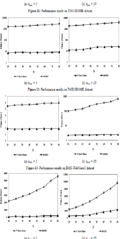
Figure 7: Efficient Implementation Components Performance Results T1014D100K dataset

Figure 8: Efficient Implementation ComponentsPerformance Results Of On Chess Dataset

Dataset Items Average Transaction Length Records

T10I4D100K 1000 10 100,000

T40I10D100K 1000 40 100,000

Chess 75 35 3196

Mushroom 119 23 8124

BMS-POS 1658 7.5 515,597

(9)

Table 1: Computational Experiments in .

Figure 14: Results of performance on BMS-POS dataset

PERFORMANCE EVALUATION OF N-Most-Miner

We play out our computational experiments using the different N-most esteems 10, 20, 30, 40, 50, 60, 70 and 80 under two kmax limits esteems, kmax = 5 ((1≤ k≤ 5) and kmax = 10 ((1≤ k≤ 10). The performance measure is the execution time of the algorithms under different N and kmax edge esteems. Figures 9-14 comes about demonstrate that the N-MostMiner beats the BOMO on both all and shut frequent itemsets mining issues, on all levels of mining edges on a wide range of meager

(10)

inadequate sort datasets when contrasted with dense sort datasets.

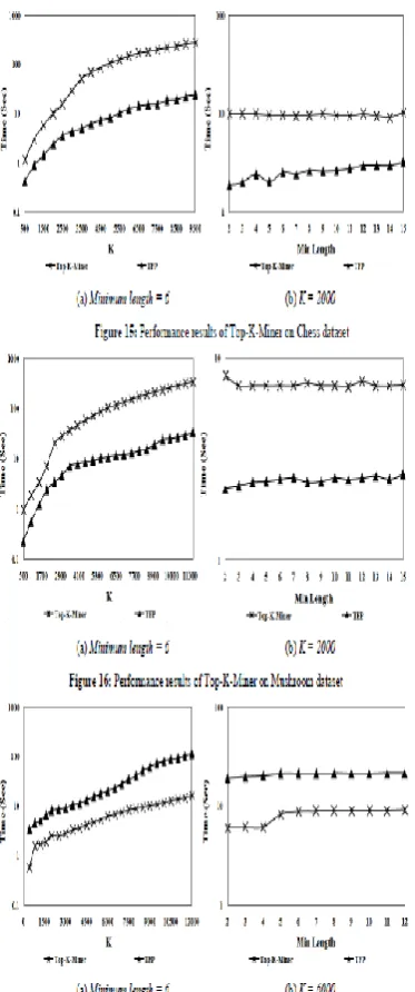
Figure 17: Performance results of Top-K-Miner on

T1014D100K dataset

PERFORMANCE EVLATUATION OF TOP-K-MINER

Our second arrangement of experiments were on mining Top-K shut frequent itemsets mining with minimum length more noteworthy than min_l edge. The experiments were performed on each dataset using two different scenarios. In to start with, we settled the minimum length and fluctuated the K esteem. While in second,

the K esteem was kept settled and minimum length was changed. Figure 15 and 16 demonstrate the performance aftereffect of TFP and Top-K-Miner on two dense sort datasets (Chess and Mushroom). Because of modest number of things and extensive normal transactional length, TFP makes a minimal initial FP-Tree, in which parcel of transactions shares a common prefix way, which helps in quick itemset frequency counting. On dense sort datasets, we note that the efficient implementation techniques of Top-K-Miner particularly 2-Itemset Pair and IPBRD does not make any significant performance impact, only frequency counting dominates the entire algorithm execution result. Figure 17 to 20 demonstrate the performance comes about on two algorithms on scanty sort datasets. As clear from the figure comes about the Top-K-Miner outflank the TFP on all levels of mining limit esteems, due to its efficient piece vector projection and implementation techniques particularly 2-Itemset Pair and IPBRD. On save datasets with huge number of things and transactions, TFP faces an indistinguishable issue from BOMO of ts initial FP-Tree construction, when ξ equivalent to zero, which backs off the entire algorithm execution.

CONCLUSION

(11)

representation approach, which is exceptionally efficient regarding candidate itemset frequency counting. For projection we present a novel piece vector projection technique PBR (anticipated piece regions), which is exceptionally efficient regarding processing time and memory requirement. A few efficient implementation techniques of N-MostMiner and Top-K-Miner are likewise presented, which we experienced in our implementation. Our experimental outcomes on benchmark datasets propose that mining interesting frequent itemsets without minimum help edge using N-MostMiner or Top-K-Miner is very efficient as far as processing time when contrasted with currently best algorithms BOMO and TFP. This demonstrates the effectiveness of our algorithm.

REFERENCE

[1] R. Agrawal and R. Srikant, “Fast Algorithms for Mining Association Rules”, In Proceedings ofinternational conference on Very Large Data Bases (VLDB), pp. 487-499, Sept. 1994. [2] R. Agrawal and R. Srikant, “Mining Sequential

Patterns”, In proceedings of international conferenceon Data Engineering (ICDE), pp. 3-14, Mar. 1995.

[3] R. Agrawal, C. Agrawal, and V. Prasad, “Depth first generation of long patterns”, In SIGKDD, 2000.

[4] J. Ayres, J. Gehrke, T. Yiu, and J. Flannick, “Sequential Pattern Mining Using Bitmaps”, In Proceedings of the Eighth ACM SIGKDD International Conference on Knowledge Discovery and Data Mining, Edmonton, Alberta, Canada, July, 2002.

[5] R. J. Bayardo, “Efficiently mining long patterns from databases”, In SIGMOD 1998: 85-93. [6] D. Burdick, M. Calimlim, and J. Gehrke,

“Mafia: A maximal frequent itemset algorithm for transactional databases”, In proceedings of International Conference of Data Engineering, pp. 443-452, 2001.

[7] Y. L. Cheung, A. W. Fu, “An FP-tree Approach for Mining N-most Interesting Itemsets”, In Proceedings of the SPIE Conference on Data Mining, 2002.

[8] G. Dong, J. Li, “Efficient mining of emerging patterns: Discovering trends and differences”,

In proceedings of 5th ACM SIGKDD international conference on Knowledge Discovery and Data Mining (KDD'99), San Diego, CA, USA, pp. 43-52, 1999.

[9] A. W. C. Fu, R. W. W. Kwong, and J. Tang, “Mining N-most Interesting Itemsets”, In proceedings of international symposium on Methodologies for Intelligent Systems (ISMIS), 2000.

[10] Proc. IEEE ICDM Workshop Frequent Itemset Mining Implementations, B. Goethals and M.J. Zaki, eds., CEUR Workshop Proc., vol. 80, Nov. 2003, http://CEUR-WS.org/Vol-90. [11] J. Han, J. Pei, and Y. Yin, “Mining frequent

patterns without candidate generation”, In proceedings ofSIGMOD, pages 1–12, 2000. [12] J. L. Koh, P. Yo, “An Efficient Approach for

Mining Fault-Tolerant Frequent Patterns based on Bit Vector Representations”, In proceedings of 10th International Conference DASFAA 2005, Beijing, China, April 17-20, 2005. [13] B. Liu, W. Hsu, and Y. Ma, “Integrating

classification and association rule mining”, In

proceedings of KDD’98, New York, NY, Aug. 1998.

[14] N. Pasquier, Y. Bastide, R. Taouil, and L. Lakhal, “Discovering frequent closed itemsets for association rules”, In 7th international conference on Database Theory, January 1999. [15] J. Pei, J. Han, H. Lu, S. Nishio, S. Tang

and D. Yang, “H-Mine: Hyper-structure mining of frequent patterns in large databases”, In proceedings of international conference on Data Mining (ICDM), pp. 441.448, 2001.

[16] R. Rymon, “Search through Systematic Set Enumeration”, In proceedings of third international conference on Principles of Knowledge Representation and Reasoning, 1992, pp. 539 –550.

[17] T. Uno, M. Kiyomi, H. Arimura, “LCM ver 3: Collaboration of Array, Bitmap and Prefix Tree for Frequent Itemset Mining”, In 1st International Workshop on Open Source Data Mining (in conjunction with SIGKDD-2005), 2005.