Robust Statistical Method for Estimating Optimal Dynamic Treatment Regimes.

ABSTRACT

ZHANG, BAQUN. Robust Statistical Method for Estimating Optimal Dynamic Treatment Regimes. (Under the direction of Anastasios Tsiatis and Marie Davidian.)

This dissertation includes two parts. In part one, we develop a new and more robust method for estimating the optimal treatment regime for a single treatment decision. A treatment regime

is a rule that assigns a treatment, among a set of possible treatments, to a patient as a function

of his/her observed characteristics, hence “personalizing” treatment to the patient. The goal is to identify the optimal treatment regime that, if followed by the entire population of patients,

would lead to the best outcome on average. Given data from a clinical trial or observational

study, for a single treatment decision, the optimal regime can be found by assuming a regression model for the expected outcome conditional on treatment and covariates, where, for a given

set of covariates, the optimal treatment is the one that yields the most favorable expected

outcome. However, treatment assignment via such a regime is suspect if the regression model is incorrectly specified. Recognizing that, even if misspecified, such a regression model defines a

class of regimes, we instead consider finding the optimal regime within such a class by finding

the regime the optimizes an estimator of overall population mean outcome. To take into account possible confounding in an observational study and to increase precision, we use a doubly robust

augmented inverse probability weighted estimator for this purpose. Simulations and application

to data from a breast cancer clinical trial demonstrate the performance of the method.

In part two, we extend the proposed method to the case of more than one treatment decisions

for the dynamic treatment regime. A dynamic treatment regime is a list of sequential decision

rules for assigning treatment based on a patient’s history. Q- and A-learning are two main approaches for estimating the optimal regime, that yielding the greatest benefit in the patient

population with respect to an outcome using data from a clinical trial or observational study.

Q-learning requires postulating regression models for the outcome, while A-learning involves models for the part of the outcome regression representing treatment contrasts and for treatment

assignment. A key concern is the impact of model misspecification; moreover, because these

methods optimize over the class of all possible regimes, the resulting rules may be too complex for practical use. We propose an alternative approach based on maximizing a doubly robust

augmented inverse probability weighted estimator for the population mean outcome over a feasible, restricted class of regimes. Simulations demonstrate the competitive performance and

©Copyright 2012 by Baqun Zhang

Robust Statistical Method for Estimating Optimal Dynamic Treatment Regimes

by Baqun Zhang

A dissertation submitted to the Graduate Faculty of North Carolina State University

in partial fulfillment of the requirements for the Degree of

Doctor of Philosophy

Statistics

Raleigh, North Carolina

2012

APPROVED BY:

Daowen Zhang Eric Laber

Anastasios Tsiatis Chair of Advisory Committee

Marie Davidian

DEDICATION

BIOGRAPHY

Zhang, Baqun was born in Hunan Province, China to parents Zhang, Decheng and Xia, Shuyun in 1982. He has a memorable childhood and school life with the love from his big family and

close friends. He graduated from Nankai University with a B.A. in Statistics. He entered the Department of Statistics at North Carolina State University (NCSU) as a graduate student in

the fall of 2006. In 2008, He received a Master of Statistics degree and he will receive his Ph.D.

ACKNOWLEDGEMENTS

First and foremost, I would like to express my deep appreciation to my advisors, Anastasios (Butch), Tsiatis and Marie Davidian. You are so talent, patient and caring, It is my fortune and

honor to be your student. I learned so much from your knowledge and expertise, this research could not be completed without your guidance and support. Hopefully, I did not disappoint

you. Words are never my strength, Gratitude is always in my heart.

I would also like to thank my committee memebers: Dr. Daowen Zhang, Dr. Lexin Li, Dr. Eric Laber, and Dr. ZhiLin Li. Thank Dr. Eric Laber for his contributions over the last year

and the recommendation letter for me when I was applying for academic positions. I would also

like to thank all faculty and staff members in our department. Their contribution and endeavor make our department to be such a great department, which is my mother department wherever

I go.

I would also like to thank all my friends, without their supports and encouragements, I was not able to go through some difficult situations.

Finally, I want to acknowledge my family. You are the meaning of everything in my life. To

TABLE OF CONTENTS

List of Tables . . . vii

List of Figures . . . x

Chapter 1 Introduction . . . 1

1.1 Robust Method for Estimating Optimal Treatment Regimes . . . 1

1.2 Robust Estimation of Optimal Dynamic Treatment Regimes for Sequential Treat-ment Decisions . . . 3

Chapter 2 Framework and Methods for Single Treatment Decision . . . 5

2.1 Framework . . . 5

2.2 Proposed Robust Method . . . 6

2.3 Marginal Structural Mean Model Approach . . . 9

Chapter 3 Empirical Studies and Applications for Single Treatment Decision. 12 3.1 Simulation Studies . . . 12

3.1.1 Main Simulation Scenario . . . 12

3.1.2 Additional Simulation Scenarios . . . 17

3.1.3 Simulation Scenarios for Comparison to Marginal Structural Mean Model Approach . . . 23

3.1.4 Summary . . . 26

3.2 Application to the NSABP Trial . . . 28

3.3 Discussion . . . 30

Chapter 4 Framework and Methods for Sequential Treatment Decisions . . . . 32

4.1 Framework . . . 32

4.2 Q- and A- Learning . . . 35

4.3 Proposed Robust Method . . . 36

Chapter 5 Empirical Studies and Applications for Sequential Treatment De-cisions . . . 41

5.1 Simulation Studies . . . 41

5.2 Application to the STAR*D Trial . . . 47

5.3 Discussion . . . 49

References. . . 51

Appendices . . . 54

Appendix A Standard Error Argument . . . 55

Appendix B Further Simulation Results, Main Paper Scenarios . . . 56

B.1 Simulation Scenarios in Main Paper Using Grid Search . . . 56

LIST OF TABLES

Table 3.1 Results for the first simulation scenario using 1000 Monte Carlo data sets with n = 500. For the true optimal regime gopt _{= g}opt

η within the classGη, (η0, η1, η2) = (−0.07,−0.71,0.71) andE{Y∗(gηopt)}= 3.71.RGµt and RGµm represent the regression method using the correct and incor-rect outcome regression models; IP W E is the proposed method using (2.2); and AIP W Eµt and AIP W Eµm are the proposed method using (2.3) and the correct and incorrect outcome regression models, respec-tively. The columns η_b0, η_b1, and η_b2 show Monte Carlo average estimates, with Monte Carlo standard deviations in parentheses. The columnQb(η_bopt)

shows Monte Carlo average and standard deviation of the estimated values of the true E{Y∗(gηopt)}, SE shows the Monte Carlo average of sandwich standard errors for this quantity, Cov. shows the coverage of 95% Wald-type confidence intervals for Q(ηopt), and Q(η_bopt) shows the Monte Carlo average and standard deviation of valuesE{Y∗(_bgoptη )}obtained using 106 Monte Carlo simulations for each data set. . . 15 Table 3.2 Results for the second simulation scenario using 1000 Monte Carlo data

sets with n = 500. For the true optimal regime gηopt within the class Gη, (η0, η1, η2) = (0.66,−0.67,0.33) andE{Y∗(goptη )}= 9.33. All other quanti-ties are analogous to those in Table 3.1, withµ1andµ2 denoting the given estimator using the misspecified models µ1(A, X;β) and µ2(A, X;β), re-spectively. . . 19 Table 3.3 Results for the discrete covariates simulation scenario using 1000 Monte

Carlo data sets with n = 500. For the true optimal regime gopt = goptη within the classGη, (η0, η1, η2) = (−0.58,0.58,−0.58) andE{Y∗(gopt)η}= 3.71. All other quantities are analogous to those in Table 3.1. . . 20 Table 3.4 Results for the randomized trial simulation scenario using 1000 Monte

Table 3.5 Results for the correct MSMM simulation scenario using 1000 Monte Carlo data sets withn= 500. For the true optimal regime gopt_=gopt

η within the class Gη, η = 2 and E{Y∗(gηopt)} = 5.50. RG represents the regression method using the posited correct outcome regression model; IP W E is our proposed method using 2.2; andAIP W E is our proposed method us-ing 2.3 and the posited correct outcome regression model. M SM.I.P k0 is the MSMM method using (2.6)-(2.7) with polynomial of degree k0.

M SM.AI.P k0 is the MSMM method using (2.8)-(2.9) with polynomial of

degreek0. The columnηbshows Monte Carlo average estimate, with Monte

Carlo standard deviation in parentheses. The columnQb(_bηopt) shows Monte

Carlo average and standard deviation of the estimated values of the true

E{Y∗(gηopt)}, andQ(ηb

opt_{) shows the Monte Carlo average and standard} de-viation of valuesE{Y∗(_bgηopt)}obtained using 106 Monte Carlo simulations for each data set. . . 25 Table 3.6 Results for the incorrect MSMM simulation scenario using 1000 Monte

Carlo data sets with n = 500. For the true optimal regime gopt = goptη within the classG_η,η = 2 andE{Y∗(gηopt)}= 5.00. All table entries are as in Table 3.5. . . 27 Table 3.7 Results of fitting the logistic outcome regression model (3.1) for the

NS-ABP data. . . 29

Table 5.1 Results for the first simulation scenario using 1000 Monte Carlo data sets with n = 500. For the true optimal regime gopt = goptη within the class

G_η,ηopt= (250,−1,360,−1)T and E{Y∗(goptη )}= 1120.IP W E,DR, and

AIP W E are the proposed methods using (4.6), (4.7), and (4.8),

respec-tively. The columns bη10,ηb11, bη20 and ηb21 show Monte Carlo average

esti-mates, with Monte Carlo standard deviations in parentheses. The column

b

E(η_bopt_{) shows Monte Carlo average and standard deviation of the} esti-mated values of the trueE{Y∗(goptη )}, SE shows the Monte Carlo average of sandwich standard errors for this quantity, Cov. shows the coverage of 95% Wald-type confidence intervals for E(ηopt_{), and E(}

b

ηopt_{) shows the} Monte Carlo average and standard deviation of values E{Y∗(gb

opt η )} ob-tained using 106 Monte Carlo simulations for each data set. . . 43 Table 5.2 Results for the second simulation scenario using 1000 Monte Carlo data

sets with n = 500. For the true optimal regime gopt = goptη within the class G_η, ηopt = (250,−1,360,−1)T and E{Y∗(gηopt)} = 1120. All other quantities are analogous to those in Table 5.1. . . 45 Table 5.3 Results for the third simulation scenario using 1000 Monte Carlo data sets

with n = 500. For the true optimal regime gopt = goptη within the class

G_η, ηopt₁ = (−0.1,0.67,0.67,−0.33)T,η₂opt = (−0.1,0.67,−0.33,0.67)T and

Table B.1 Results for the first simulation scenario using 1000 Monte Carlo data sets with n = 500 using the grid search. For the true optimal regime

gopt = goptη within the class Gη, (η0, η1, η2) = (−0.07,−0.71,−0.71) and

E{Y∗(gηopt)} = 3.71. RGµt and RGµm represent the regression method using the correct and incorrect outcome regression models; IP W E is the proposed method using 2.2; andAIP W Eµt andAIP W Eµm are the pro-posed method using 2.3 and the correct and incorrect outcome regression models, respectively. The columnsη_b0,ηb1, andηb2 show Monte Carlo

aver-age estimates, with Monte Carlo standard deviations in parentheses. The columnQb(η_bopt) shows Monte Carlo average and standard deviation of the

estimated values of the trueE{Y∗(gηopt)}, SE shows the Monte Carlo aver-age of sandwich standard errors for this quantity, Cov. shows the coveraver-age of 95% Wald-type confidence intervals forQ(ηopt), and Q(η_bopt) shows the Monte Carlo average and standard deviation of values E{Y∗(g_bηopt)} ob-tained using 106 Monte Carlo simulations for each data set. . . 58 Table B.2 Results for the second simulation scenario using 1000 Monte Carlo data

sets with n= 500 using the grid search. For the true optimal regime goptη within the class Gη, (η0, η1, η2) = (0.66,−0.67,0.33) and E{Y∗(gηopt)} = 9.33. All other quantities are analogous to those in Table B.1, withµ1 and

µ2 denoting the given estimator using the misspecified modelsµ1(A, X;β) and µ2(A, X;β), respectively. . . 61 Table B.3 Results for the first simulation scenario using 1000 Monte Carlo data sets

with n = 200. For the true optimal regime gopt = goptη within the class

Gη, (η0, η1, η2) = (−0.07,−0.71,−0.71) andE{Y∗(goptη )}= 3.71. All other quantities are analogous to those in Table B.1. . . 62 Table B.4 Results for the second simulation scenario using 1000 Monte Carlo data

sets with n = 200. For the true optimal regime gηopt within the class Gη, (η0, η1, η2) = (0.66,−0.67,0.33) and E{Y∗(gηopt)} = 9.33. All other quan-tities are analogous to those in Table B.1, with µ1 and µ2 denoting the given estimator using the misspecified modelsµ1(A, X;β) andµ2(A, X;β), respectively. . . 63 Table B.5 Results for the first simulation scenario using 1000 Monte Carlo data sets

with n = 1000. For the true optimal regime gopt _{= g}opt

η within the class

Gη, (η0, η1, η2) = (−0.07,−0.71,−0.71) andE{Y∗(goptη )}= 3.71. All other quantities are analogous to those in Table B.1. . . 63 Table B.6 Results for the second simulation scenario using 1000 Monte Carlo data

sets with n = 1000. For the true optimal regime gηopt within the class

LIST OF FIGURES

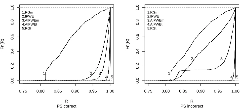
Figure 3.1 Empirical cdfs across 1000 Monte Carlo data sets using correct and incor-rect propensity score (PS) models of the quantities Q(_bηopt_)/E{Y∗_(gopt

η )} for each estimator for the first simulation scenario. RGt and RGm denote the regression estimator with correct and misspecified model µ(A, X;β), respectively; AIPWEt and AIPWEm denote the estimator based on (2.3) with correct and misspecified model µ(A, X;β), respectively; and IPWE denotes the estimator based on (2.2). . . 16 Figure 3.2 Empirical cdfs across 1000 Monte Carlo data sets using correct and

incor-rect propensity score (PS) models of the quantities Q(bη

opt_)/E{Y∗_(gopt η )} for each estimator for the second simulation scenario. RG1 and RG2 denote the regression estimator using incorrect models µ1(A, X;β) and

µ2(A, X;β), respectively; AIPWE1 and AIPWE2 denote the estimator based on (2.3) usingµ1(A, X;β) andµ2(A, X;β), respectively; and IPWE denotes the estimator based on (2.2). . . 18 Figure 3.3 Empirical cdfs across 1000 Monte Carlo data sets with n = 500

us-ing correct and incorrect propensity score (PS) models of the quantities

Q(_bηopt)/E{Y∗(ηoptη )}for each estimator for the discrete covariates simula-tion scenario. RGt and RGm denote the regression estimator with correct and misspecified model µ(A, X;β), respectively; AIPWEt and AIPWEm denote the estimator based on (2.3) with correct and misspecified model

µ(A, X;β), respectively; and IPWE denotes the estimator based on (2.2). 21 Figure 3.4 Empirical cdfs across 1000 Monte Carlo data sets withn= 500 using

cor-rect propensity score (PS) models of the quantities Q(η_bopt)/E{Y∗(ηηopt)} for each estimator for the randomized trial simulation scenario. RGt and RGm denote the regression estimator with correct and misspecified model

µ(A, X;β), respectively; AIPWEt and AIPWEm denote the estimator based on (2.3) with correct and misspecified model µ(A, X;β), respec-tively; and IPWE denotes the estimator based on (2.2). . . 24 Figure 3.5 (a) Estimated optimal treatment regimes of the formI(age≥η0+η1LPR)

using the regression estimator (RG), the estimator based on (2.2) (IPWE), and the estimator based on (2.3) (AIPWE). (b) The regime identified by Fisher et al., (1983) and Gail and Simon (1985) (solid lines) and optimal regimes of the form 1 −I(age < η0 and PR < η1) estimated based on (2.2) (dotted-dashed lines) and (2.3) (long dashed lines). . . 30

Figure B.1 Empirical cdfs across 1000 Monte Carlo data sets using correct and incor-rect propensity score (PS) models of the quantities Q(η_bopt_)/E{Y∗_(ηopt

Figure B.2 Empirical cdfs across 1000 Monte Carlo data sets using correct and incor-rect propensity score (PS) models of the quantities Q(η_bopt_)/E{Y∗_(ηopt

η )} for each estimator for the second simulation scenario. RG1 and RG2 denote the regression estimator with incorrect models µ1(A, X;β) and

µ2(A, X;β), respectively; AIPWE1 and AIPWE2 denote the estimator based on (2.3) usingµ1(A, X;β) andµ2(A, X;β), respectively; and IPWE denotes the estimator based on (2.2). . . 60 Figure B.3 Empirical cdfs across 1000 Monte Carlo data sets with n = 200

us-ing correct and incorrect propensity score (PS) models of the quantities

Q(_bηopt)/E{Y∗(ηoptη )}for each estimator for the first simulation scenario. RGt and RGm denote the regression estimator with correct and misspec-ified model µ(A, X;β), respectively; AIPWEt and AIPWEm denote the estimator based on (2.3) with correct and misspecified modelµ(A, X;β), respectively; and IPWE denotes the estimator based on (2.2). . . 62 Figure B.4 Empirical cdfs across 1000 Monte Carlo data sets with n = 200

us-ing correct and incorrect propensity score (PS) models of the quanti-ties Q(η_bopt)/E{Y∗(ηηopt)} for each estimator for the second simulation scenario. RG1 and RG2 denote the regression estimator with incorrect modelsµ1(A, X;β) andµ2(A, X;β), respectively; AIPWE1 and AIPWE2 denote the estimator based on (2.3) using µ1(A, X;β) and µ2(A, X;β), respectively; and IPWE denotes the estimator based on (2.2). . . 64 Figure B.5 Empirical cdfs across 1000 Monte Carlo data sets with n = 1000

us-ing correct and incorrect propensity score (PS) models of the quantities

Q(bη

opt_)/E{Y∗_(ηopt

η )}for each estimator for the first simulation scenario. RGt and RGm denote the regression estimator with correct and misspec-ified model µ(A, X;β), respectively; AIPWEt and AIPWEm denote the estimator based on (2.3) with correct and misspecified modelµ(A, X;β), respectively; and IPWE denotes the estimator based on (2.2). . . 65 Figure B.6 Empirical cdfs across 1000 Monte Carlo data sets with n = 1000

us-ing correct and incorrect propensity score (PS) models of the quanti-ties Q(ηb

opt_)/E{Y∗_(ηopt

Chapter 1

Introduction

In this dissertation, we study two topics. First, using semiparametric theory and causal infer-ence framework, in Chapters 2 and 3 we develop a robust method for estimating the optimal

treatment regime for a single treatment decision. Second, in Chapters 4 and 5 we extend the

proposed method to the case of more than one treatment decisions for the dynamic treatment regime. Separate sets of notations are used for these two topics.

1.1

Robust Method for Estimating Optimal Treatment Regimes

The area of personalized medicine, which is focused on making treatment decisions for an in-dividual patient based on his/her clinical, genomic, and other information, is of considerable

current interest. In the simplest case of a single treatment decision, there may be several

treat-ment options, and formalizing this objective involves defining a decision rule, or regime, that takes as input an individual’s characteristics and dictates the treatment he/she should receive

from among the options available. The optimal regime is that leading to the greatest benefit overall in the patient population; i.e., if followed by the entire population, would result in the

most favorable clinical outcome on average.

Deducing optimal treatment regimes using data from a clinical trial or observational study can be informed by identifying patient covariates that exhibit a qualitative interaction with

treatment assignment in a statistical model for the outcome of interest; i.e., an interaction

in which the treatment effect changes direction depending on covariates. For example, Gail and Simon (1985) considered data from a trial conducted by the National Surgical Adjuvant

Breast and Bowel Project (NSABP) comparing L-phenylalanine mustard and 5-fluorouracil

(PF) to PF plus tamoxifen (PFT) in patients with primary operable breast cancer and positive nodes (Fisher et al., 1983). The study investigators found “evidence for a heterogeneity in

Simon proposed a test for qualitative interaction based on partitioning the data into subsets

using covariate values and concluded on its basis that young patients (age < 50 years) with progesterone receptor levels<10 femtomole/mg cytosol protein (fmol) achieve better outcomes

on PF whereas other patients do better on PFT. However, this approach does not target formally

the goal of identifying the optimal regime.

More recently, there has been vigorous research on methods for estimating optimal treatment

regimes based on data from clinical trials or observational studies, where a single decision or a

series of sequential decisions may be involved (Murphy, 2003; Robins, 2004; Moodie, Richard-son, and Stephens, 2007; Robins, Orellana, and Rotnitzky, 2008; Brinkley, Tsiatis, and Anstrom,

2009; Zhao, Kosorok, and Zeng, 2009; Henderson, Ansell, and Alshibani, 2010; Orellana,

Rot-nitzky, and Robins, 2010; Gunter, Zhu, and Murphy, 2011). In the setting of a single treatment decision, much of this work involves postulating a model for the regression of outcome on

treat-ment assigntreat-ment and covariates and then assigning treattreat-ment for a patient according to which

treatment yields the best estimated mean outcome based on the model and given the patient’s particular covariate values. However, this approach is clearly predicated on whether or not the

assumed model is correctly specified.

In the first part of this dissertation, we focus on the case of a single decision and take an al-ternative view, considering such a posited regression model as a mechanism for defining a class

of treatment regimes but recognizing that the model may in fact be misspecified. Assuming without loss of generality that larger outcomes are preferred, we then base estimation of the

optimal regime on maximizing directly an estimator for the overall population mean outcome

under regimes in the class. Specifically, we maximize across all regimes in the class a suitable doubly robust augmented inverse probability weighted estimator (e.g., Bang and Robins, 2005).

This estimator takes account of possible confounding in the case of data from an observational

study via estimated propensity scores and exploits the postulated outcome regression relation-ship to gain precision. As we demonstrate, this approach leads to estimated optimal regimes

that can achieve comparable performance to those based on correctly specified outcome

regres-sion models; outperform those based on simpler mean estimators; and, because of the double robustness property, are protected from misspecification of either the propensity score model

or the outcome regression model.

In Section 2.1, we define a framework in which we may formalize the problem. We introduce the proposed methods and describe the marginal structural mean model (MSMM) approach of

Robins et al. (2008) and Orellana et al. (2010) in our situation of a single treatment decision

1.2

Robust Estimation of Optimal Dynamic Treatment Regimes

for Sequential Treatment Decisions

Treatment of patients with chronic disease involves a series of decisions, where the clinician determines the treatment to be administered next to a patient based on all information available

on the patient up to that point. A dynamic treatment regime is a set of sequential decision rules,

each corresponding to a key decision point in the disease process, where each rule takes the available information as input and yields the treatment action to be taken from among the

available options. The optimal dynamic treatment regime is the set of rules that would yield the most favorable outcome on average if followed by the entire patient population.

Following from developments on reinforcement learning for sequential decision-making in

computer science, Q-learning and A-learning are two main approaches proposed to estimate the optimal dynamic treatment regime based on data from a clinical trial or observational

study. Q-learning (Watkins, 1989; Watkins and Dayan, 1992) involves postulating at each

deci-sion point regresdeci-sion models for the outcome of interest as a function of patient information to that point. A-learning (Murphy, 2003; Blatt, Murphy and Zhu, 2004) involves instead positing

models for only the part of the outcome regression having to do with contrasts among

treat-ments and for treatment assignment at each decision point. Both methods are implemented through a backward recursive fitting procedure based on a dynamic programming algorithm

(Bather, 2000). Under certain assumptions and correct specification of these models, Q- and

A-learning will lead to consistent estimation of the optimal treatment regime. See Rosthøj et al. (2006), Murphy et al. (2007), Zhao, Kosorok and Zeng (2009), Henderson, Ansell, and

Al-shibani (2010) for applications of Q- and A-learning. Other methods for estimating optimal

regimes are discussed by Robins (2004), Moodie, Richarson and Stephens (2007), Robins, Orel-lana and Rotnitzky (2008), Almirall, Ten Have and Murphy (2010), and OrelOrel-lana, Rotnitzky,

and Robins (2010).

An obvious concern with both Q- and A-learning is the effect of model misspecification on credibility of the estimated optimal regime. Moreover, as these methods deduce the optimal

regime across the class of all possible regimes, the estimated optimal rules may be complicated

functions of possibly high-dimensional patient information that are difficult to interpret or implement and hence unappealing to clinicians wary of “black box” approaches.

Given these drawbacks, we focus on a restricted class of treatment regimes indexed by a finite number of parameters, where the form of regimes in the class may be derived from posited

regression models or prespecified to depend on key subsets of patient information on grounds

of interpretability or cost. In the first part of the dissertation we propose an approach for esti-mating the optimal regime within such a restricted class for a single treatment decision based

the population mean outcome over all regimes in the class, assuming without loss of

gener-ality that larger outcomes are preferred. Via the double robustness property, the estimated optimal regimes enjoy protection against model misspecification and comparable or superior

performance to competing methods.

In the second part of the dissertation, we adapt this approach to the case of two or more sequential decision points, which is considerably more involved and is based on casting the

problem as one of monotone coarsening (Tsiatis, 2006, chapter 7). The new methods lead to

estimated optimal regimes that achieve performance comparable to that of those derived via Q- or A-learning under correctly specified models and offer protection against misspecification.

In Section 4.1, we define a framework in which we may formalize the problem, and we review

Q- and A-learning in Section 4.2. We introduce the proposed methods in Section 4.3, and we demonstrate their performance in simulation studies in Section 5.1 and by application to a

Chapter 2

Framework and Methods for Single

Treatment Decision

2.1

Framework

Consider a clinical trial or observational study withn subjects sampled from the patient

pop-ulation of interest. Suppose there are two treatment options, e.g., control and experimental treatment in a clinical trial, and letA, taking values 0 or 1 in accordance with the two options,

denote observed treatment received. Let X be a vector of subject characteristics ascertained

prior to treatment, and letY be the observed outcome of interest, where, as in Section 1.1, we assume larger values of Y are preferred. The observed data are then (Yi, Ai, Xi), i= 1, . . . , n, independent and identically distributed (iid) acrossi. The goal is to use these data to estimate

the optimal treatment regime, defined as follows.

In this context, a treatment regime is a functiong that maps values of X to{0,1}, so that

a patient with covariate value X = x would receive treatment 1 if g(x) = 1 and treatment 0

if g(x) = 0. A simple example for scalar X is g(X) = I(X < 50). To identify formally the optimal such treatment regime, we define potential outcomes Y∗(0) and Y∗(1), representing the outcomes that would be observed were a subject to receive treatment 0 or 1, respectively.

As is customary (e.g., Rubin, 1978), we assume that Y =Y∗(1)A+Y∗(0)(1−A), so that the observed outcome is the potential outcome that would be seen under the treatment actually

received. We also assume {Y∗(0), Y∗(1)} independent of A conditional on X; i.e., that there are no unmeasured confounders. This is trivially true in a randomized clinical trial but is an

unverifiable assumption in an observational study (e.g., Robins, Hern´an, and Brumback, 2000).

Thus, for a = 0,1, E{Y∗(a)} represents the overall population mean were all patients in the population to receive treatmenta, and, under these assumptions, it is straightforward to deduce

to the marginal distribution ofX.

Note that, for arbitrary treatment regime g, we can thus define the potential outcome

Y∗(g) =Y∗(1)g(X) +Y∗(0){1−g(X)} that would be observed if a randomly chosen subject from the population were to be assigned treatment according to g, where we suppress the

dependence of Y∗(g) onX. If G is the class of all such treatment regimes, then we may define the optimal regime,gopt, as the one leading to the largest value of E{Y∗(g)} amongg∈ G; i.e.,

gopt(X) = arg maxg∈G E{Y∗(g)}. Under the above assumptions, writing µ(a, X) = E(Y|A =

a, X),a= 0,1, it is straightforward to show that

E{Y∗(g)}=EX[µ(1, X)g(X) +µ(0, X){1−g(X)}],

and hence the optimal treatment regime is given by

gopt(X) =I{µ(1, X)> µ(0, X)};

i.e., the optimal regime assigns the treatment that yields the larger mean outcome conditional

on the value of X. Here, the strict inequality follows from the convention that, in the event

µ(1, X) =µ(0, X) and viewing treatments 0 and 1 as control and experimental, respectively, a

conservative strategy would be to prefer the control.

2.2

Proposed Robust Method

To exploit the developments in the previous section, an obvious approach is to posit a

regres-sion model for µ(A, X) = E(Y|A, X), for example, a parametric model µ(A, X;β) for finite-dimensional parameter β, and to estimate β by βb obtained via some appropriate method;

e.g., least or generalized least squares. Assuming the model is correctly specified, so that

µ(A, X) = µ(A, X;β0) for some β0, the optimal regime is then g(X, β0), where g(X, β) =

I{µ(1, X, β) > µ(0, X, β)}, and it is natural to estimate the optimal treatment regime by

b

goptreg(X) =g(X,βb), which we denote as the regression estimator. An obvious estimator for the

overall mean outcome under the optimal regime,E{Y∗(gopt)}, is then

n−1

n

X

i=1

[µ(1, Xi,βb)g_bregopt(X_i) +µ(0, X_i,βb){1−_bgopt_reg(X_i)}]. (2.1)

Of course, whether or not_bgregopt is a credible estimator for the true optimal regime gopt depends critically on whether or not the modelµ(A, X;β) is correct. If it is not, then treatment

A posited model µ(A, X;β), whether correct or not, may be viewed as defining the class

of treatment regimes indexed by β, Gβ, say, with elements of the form g(X, β). In fact, in many instances, only a subset of elements of X and β may define the regime, and the class

may be simplified. E.g., if µ(A, X;β) = exp{β0+β1X1+β2X2+A(β3+β4X1+β5X2)}, it is

straightforward to show that elements in the class are of the form I(β3+β4X1+β5X2 > 0), which may be rewritten in terms ofη0 =−β3/β5 and η1=−β4/β5 as either I(X2 > η0+η1X1)

orI(X2 < η0+η1X1) depending on the sign of β5. This suggests considering directly regimes

of the form gη(X) = g(X, η) in a class Gη, say, indexed by a parameter η. In the event the regimes inG_η are derived from a regression modelµ(A, X;β), as above, η=η(β) is a many-to-one function of β, andGη will containgopt ifµ(A, X;β) is correct. Thus, estimating the value

ηopt= arg maxηE{Y∗(gη)} defining the regimegηopt(X) =g(X, ηopt) will yield an estimator for

gopt. For complex regression models involving high-dimensionalX, the resulting regimes may be difficult to interpret or implement broadly; e.g., if some elements ofXare not routinely collected

in practice. Then, alternatively, it may be desirable to specify directly a class of regimes indexed by a parameter η and depending on a key subset of elements of X based on clinical practice,

cost, and interpretability, without reference to a regression model. In this case, gopt may or may not be in Gη. However, although the regime gηopt defined by ηopt may not be the same as

gopt, when attention focuses on the feasible class G_η, estimation of goptη is still of considerable interest. When the regimes in Gη are derived from a misspecified regression model, η(βb) may

or may not converge in probability to ηopt_{, and the resulting estimator for the optimal regime} based onβbcan exhibit very poor performance, as we demonstrate in Section 3.1 (see also Qian

and Murphy, 2011, Section 3), suggesting the need for an alternative approach to estimation of

ηopt_.

Based on these considerations, our approach is to identify an estimator for E{Y∗(gη)} and to maximize it directly in η to obtain an estimator ηb

opt _{for η}opt _{and thus an estimator}

b

goptη (X) =g(X,bη

opt_{) forg}opt

η . To this end, for fixedη, letCη =Ag(X, η) + (1−A){1−g(X, η)}, so that, whenCη = 1,Y =Y∗(gη), so thatY∗(gη) is observed; otherwise, ifCη = 0, thenY∗(gη) is “missing.” By analogy to a standard missing data problem as in Cao et al. (2009), we can conceive of “full data” {Y∗(gη), X} and “observed data” {Cη, CηY∗(gη), X} = {Cη, CηY, X}. Note thatY∗(gη) is a function of {Y∗(1), Y∗(0), X}, andCη is a function of{A, X}. Under the assumptions in Section 2.1, as {Y∗(1), Y∗(0)} is independent ofA conditional onX, it follows that Y∗(gη) is independent of Cη conditional on X, which corresponds to the assumption of “missing at random,” so that pr{Cη = 1|Y∗(gη), X}= pr(Cη = 1|X). Letπ(X) = pr(A= 1|X) denote the propensity score for treatment. It is then straightforward to obtain pr(Cη = 1|X) =

πc(X;η) =π(X)g(X, η) +{1−π(X)}{1−g(X, η)}.

In a randomized trial,π(X) is known and is ordinarily a constant; in an observational study,

such as the logistic regression modelπ(X;γ) = exp(γTX˜)/{1 + exp(γTX˜)}, ˜X= (1, XT)T; and estimateγ via the maximum likelihood (ML) estimatorbγ based on the iid (Ai, Xi),i= 1, . . . , n.

We may thus estimateπc(X;η) by πc(X;η,bγ) =π(X;bγ)g(X, η) +{1−π(X;bγ)}{1−g(X, η)}.

Note that, although the restricted classG_η may depend on X only through a specific subset of its elements, in an observational study the propensity score modelπ(X, γ) should be developed based on all of X to ensure that confounding is addressed.

Following the missing data analogy, we now identify estimators for E{Y∗(gη)}. For fixedη, the simple inverse probability weighted estimator (IPWE) is given by

IP W E(η) =n−1

n

X

i=1

Cη,iYi

πc(Xi;η,bγ)

=n−1

n

X

i=1

Cη,iYi

π(Xi;bγ)

Ai_{1−π(Xi;

b

γ)}1−Ai. (2.2) As in the missing data context, the estimator (2.2) is consistent for E{Y∗(gη)} ifπ(X;γ), and henceπc(X;η, γ), is correctly specified, but may not be otherwise.

Following Robins, Rotnitzky, and Zhao (1994) and Cao et al. (2009), an alternative estimator that offers protection against such misspecification and improved efficiency is the doubly robust

augmented inverse probability weighted estimator (AIPWE)

AIP W E(η) =n−1

n

X

i=1

Cη,iYi

πc(Xi;η,bγ)

−Cη,i−πc(Xi;η,bγ)

πc(Xi;η,bγ)

m(Xi;η,βb)

. (2.3)

In (2.3),m(X;η, β) =µ(1, X, β)g(X, η) +µ(0, X, β){1−g(X, η)}is a model forE{Y∗(gη)|X}=

µ(1, X)g(X, η) +µ(0, X){1−g(X, η)}, where µ(A, X;β) is a model for E(Y|A, X), and βb is

an appropriate estimator for β as before. The estimator (2.3) possesses the double robustness

property; i.e., it is consistent for E{Y∗(gη)} if either of π(X;γ), and hence, πc(X;η, γ), or

µ(A, X;β), but not both, is misspecified. Note that, while the regression estimator (2.1) may

be used to estimateE{Y∗(gη)}for any arbitrary gη, regardless of whether or not gη is derived from a regression model, its consistency hinges critically on correct specification of a model for

E(Y|A, X). Likewise, the estimator (2.2) requires a correct model forπ(X;γ). Thus, relative to

these approaches, (2.3) offers protection against mismodeling of these key quantities. Finally, as

shown by Robins et al. (1994), the second term in (2.3) “augments” the estimatorIP W E(η) so as to increase asymptotic efficiency; ifπ(X;γ) is correctly specified, then the efficient estimator

of form (2.3) is obtained when the regression model is also correct. If µ(A, X;β) is correctly

specified, the regression estimator may achieve greater large-sample precision; however, as we demonstrate in Section 3.1, the gain can be modest.

An estimator forηoptand hence forgoptη may be obtained by maximizingAIP W E(η) in (2.3) inη to obtainηb

opt _{and thus}

b

gηopt(X) =g(X,ηb

AIP W E(_bηopt). Analogous estimators based onIP W E(η) may also be obtained; in Section 3.1, we show that those based onAIP W E(η) exhibit superior performance.

Standard errors for these estimators for E{Y∗(gηopt)} may be obtained under regularity conditions based on an argument sketched in Appendix A. Letting Q(η) = E{Y∗(gη)} as a function of η, and denoting either estimator by Qb(η) for arbitraryη, it is shown that

n1/2{Qb(η_bopt)−Q(ηopt)}=n1/2{Qb(ηopt)−Q(ηopt)}+o_p(1), (2.4)

so that the asymptotic variance of the left hand side of (4.9) can be approximated by that

of the leading term on the right, which can be estimated by the usual sandwich technique

(Stefanski and Boos, 2002).

2.3

Marginal Structural Mean Model Approach

In the situation of a series of sequential decisions, Robins et al. (2008) and Orellana et al. (2010)

also consider treatment regimes gη, say, in a restricted class Gη indexed by a parameter η and propose methods to estimate the optimal regime within the class. These authors motivate their

approach in the context of HIV infection, where the goal is to determine the optimal threshold CD4 countηsuch that, if at any point a subject were to exhibit CD4 count belowη, he/she would

be administered antiretroviral therapy. Similar to our approach, the optimal ηmaximizes Q(η)

for some outcome of interest. In this more complex time-dependent setting, however,Q(η) may be difficult to estimate because the number of subjects in the data treated in accordance withgη for any fixedηmay be quite small. Accordingly, in contrast to our approach, where we maximize

an estimatorQb(η) inη directly, these authors posit a marginal structural mean model forQ(η),

M(η, τ), say, in terms of a parameterτ; e.g., a quadratic modelM(η, τ) =τ0+τ1η+τ2η2. The

estimator_bτ is obtained via (augmented) inverse probability weighted estimating equations; and

the optimalη is then estimated as arg maxηM(η,τb).

Next we describe an approach to implementation of the marginal structural mean model

(MSMM) approach of Robins et al. (2008) and Orellana et al. (2010) in our situation of a single

treatment decision. We use this approach to implementation of these methods in the simulations reported in section 3.1.3.

For definiteness, we consider MSMMs for Q(η) of the form

M(η, τ) =τ0+

k0

X

k=1

τkηk; (2.5)

be the restricted class of regimes under consideration.

A first approach to estimation ofτ is to solve inτ the inverse probability weighted estimating equation

n

X

i=1

Z

Gη

C_η,i

πc(Xi;η,bγ)

∂M(η, τ)

∂τ {Yi−M(η, τ)}dv(η) = 0, (2.6)

where all quantities are defined as in the main paper, anddv(η) is a mass function that weights

across the different regimes gη in Gη. For example, in the simulations in section 3.1.3, we consider regimes withη in the interval [0,4] and a discrete partition of this interval defined by the sequence ηj, j = 1, . . . , m, with step size 0.01, so that dv(η) puts point mass 1/mat each

ηj. In this case, (2.6) becomes n

X

i=1 m

X

j=1

Cηj,i

πc(Xi;ηj,bγ)

∂M(ηj, τ)

∂τ {Yi−M(ηj, τ)}= 0. (2.7)

To solve (2.7) inτ to obtain the estimatorτb, we create an artificial data set of sizeT =nm, with

each subject i = 1, . . . , n contributing m observations (Yi, Xi, η1),(Yi, Xi, η2), . . . ,(Yi, Xi, ηm). The estimator of τ is then computed as the weighted least squares estimator from the fit of

the regression model M(η, τ) = τ0 +Pk0_k=1τkηk to the artificial data set of size T, taking all observations to be independent and weighting each artificial observation (Yi, Xi, ηj) with weights

Wij =Cηj,i/πc(Xi;ηj,γb). Given bτ, the estimated optimal regime may be found by estimating

the optimalη, which is accomplished by finding arg maxηM(η,bτ). In the simulations of section

3.1.3, we used optimizein R to find the value at which M(η,τ_b) =τ_b0+Pk0k=1bτkη

k _{attains its} maximum on [0,4].

Efficiency gains may be made by using instead an augmented inverse probability weighted

estimating equation, which in this context is given by

n

X

i=1

Z

Gη

∂M(η, τ)

∂τ

_C

η,iYi

πc(Xi;η,bγ)

−Cη,i−πc(Xi;η,bγ)

πc(Xi;η,bγ)

m(Xi;η,βb)−M(η, τ)

dv(η) = 0,

(2.8)

where all quantities are as in the main paper. Using the same strategy as for (2.6) to implement

(2.8), (2.8) becomes

n

X

i=1 m

X

j=1

∂M(ηj, τ)

∂τ

_C

ηj,iYi

πc(Xi;ηj,bγ)

− Cηj,i−πc(Xi;ηj,bγ)

πc(Xi;ηj,bγ)

m(Xi;ηj,βb)−M(η_j, τ)

= 0.

To solve (2.9) inτ to obtain the estimator_bτ, we let

e

Yi=

Cηj,iYi

πc(Xi;ηj,bγ)

−Cηj,i−πc(Xi;ηj,bγ)

πc(Xi;ηj,bγ)

m(Xi;ηj,βb)

fori= 1, . . . , n and create an artificial data set of sizeT =nm, with each subjecti= 1, . . . , n

contributing m observations (Ye_i, η1), . . . ,(Ye_i, ηm). The estimator for τ may then be computed

as the ordinary least squares estimator from the fit of the regression model M(η, τ) = τ0+

Pk0

Chapter 3

Empirical Studies and Applications

for Single Treatment Decision

3.1

Simulation Studies

We have carried out several simulation studies to evaluate the performance of the proposed

methods, each involving 1000 Monte Carlo data sets. Further results are presented in Appendices B.

3.1.1 Main Simulation Scenario

For the first scenario, for each data set, we generated n = 500 observations (Yi, Ai, Xi), i =

1, . . . , n, whereXi= (Xi1, Xi2)T and Xi1 and Xi2 were independent and uniformly distributed

on (−1.5,1.5); given Xi, Ai were Bernoulli with success probability satisfying logit{pr(A = 1|X)} = −1.0 + 0.8X₁2+ 0.8X₂2, logit(u) = log{u/(1−u)}; and outcomes were generated as

Yi =µ(Ai, Xi) +ifori standard normal andµ(A, X) = exp{2.0−1.5X12−1.5X22+ 3.0X1X2+

A(−0.1−X1+X2)}. It is straightforward to deduce that the optimal treatment regimegopt(X) =

I(X2 > X1+ 0.1), a hyperplane in two dimensional space. Via Monte Carlo simulation with 106

replicates, we obtained E{Y∗(gopt_{)} = 3.71, E{Y}∗_{(0)} = 3.02, and E{Y}∗_{(1)} = 3.14. Thus,}

while the strategy of administering treatment 1 to the entire population results in improved

mean outcome relative to giving treatment 0 to the entire population, there is added benefit to assigning treatment via gopt, which leads to an 18% increase in mean outcome over treatment 1.

To estimate the optimal regime, we considered the regression estimator and the estima-tors based on maximizing IP W E(η) in (2.2) and AIP W E(η) in (2.3) in η, respectively,

we considered two posited outcome regression models, which we denote as µt(A, X;β) = exp{β0+β1X12+β2X22+β3X1X2+A(β4+β5X1+β6X2)}, corresponding to the correct specifica-tion; andµm(A, X;β) =β0+β1X1+β2X2+A(β3+β4X1+β5X2), which is misspecified. We esti-matedβin each model by least squares. Forπ(X;γ), we considered the correctly specified model

logit{πt(X;γ)}=γ0+γ1X12+γ2X22and an incorrect version logit{πm(X;γ)}=γ0+γ1X1+γ2X2, both of which were fitted via ML. Both outcome regression models define a class of treatment

regimes G_η = {I(η0 +η1X1+η2X2 > 0)}, so that clearly gopt ∈ Gη. Expressed in this form, regimes in Gη do not have a unique representation. Rather than achieving this by taking the coefficient of one of the covariates equal to 1 and redefiningη, as in the discussion in Section 2.2,

which yields easily interpretable regimes, for computational convenience in automating the

sim-ulations we instead equivalently achieved uniqueness by imposingkη k= (ηTη)1/2 = 1. In this case,gopt∈ G_η corresponds to η= (η0, η1, η2)T = (−0.07,−0.71,0.71)T.

BothIP W E(η) and AIP W E(η) are non-smooth functions inη; accordingly, the use of

tra-ditional optimization methods to maximize these quantities inη may be problematic. Accord-ingly, we used two approaches to maximization of these quantities: a grid search, as described in

Appendix B, and the genetic algorithm discussed by Goldberg (1989) and implemented in the

rgenoud package in R (Mebane and Sekhon, 2011). As noted in the documentation, the latter

“combines evolutionary algorithm methods with a derivative-based quasi-Newton approach” to

address difficult such optimization problems. In our context, we have found this approach to be computationally efficient in higher dimensions, whereas a direct grid search quickly becomes

infeasible for dimensions greater than two. In our implementation using the genoud function,

we adopted the default settings of all arguments except we took max=TRUE; optim.method =

Nelder-Mead, recommended in the documentation for discontinuous objective functions; and

pop.size = 3000, which we determined to be sufficiently large to achieve satisfactory results

via preliminary testing. We took starting.values = c(0,0,0), and set the Domains matrix to be the 3×2 matrix with columns (−1,−1,−1)T _{and (1,1,1)}T_{, where, each row corresponds} to lower and upper bounds on each element ofη, so that the algorithm searched in this region.

As above, to identify a unique estimatedηopt, we imposed the restrictionkηk= 1, normalizing the value of η_bopt obtained from genoud for each Monte Carlo data set. We provide further discussion of selection of these tuning parameters in Appendix B.

Table 3.1 shows the results using the genetic algorithm to carry out the maximization for the proposed estimators; results using the grid search were almost identical and are given in

Appendix B. For the regression estimators, we reportη(βb). For the proposed estimators based

on (2.2) and (2.3), results are shown using both correct and incorrect models for the propensity score and outcome regression in different combinations. In accordance with the definitions of

Q(η) and Qb(η), Qb( b

approach does at estimating the true achievable mean outcome under the true optimal regime.

In contrast, Q(ηb

opt_{) is a measure of the actual performance of the estimated optimal regime} itself. Namely, for each Monte Carlo data set, the true mean outcome that would be achieved

if each estimated optimal regime were followed by the entire population was determined by

simulation, and the values in this column are the Monte Carlo average (standard deviation) of these simulated quantities. Hence, the values in this column, when compared to the true

E{Y∗(goptη )} = 3.71, reflect the extent to which the estimated optimal regime can achieve the performance of the true optimal regime. We also present Monte Carlo coverage probabilities for 95% Wald confidence intervals for Q(ηopt) constructed using Qb(_bηopt) and standard errors

obtained as described in Section 2.2.

To obtain a graphical depiction of the performance of the estimated optimal regimes, we calculated the ratio Q(η_bopt)/E{Y∗(gopt)} = Q(_bηopt)/E{Y∗(gηopt)} for each Monte Carlo data set, which gives the proportion of benefit the estimated regime can achieve if used in the entire

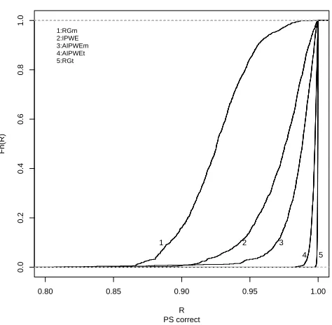
population relative to using the true optimal regime. The empirical cumulative distribution function (cdf) of these ratios for each estimator is presented in Figure 3.1; by definition, “good”

estimators should admit empirical cdfs that concentrate at 1.00.

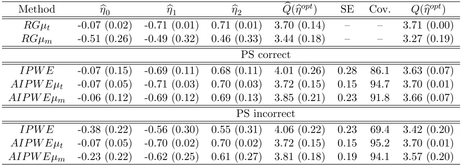
From Table 3.1, the regression estimator based on a postulated outcome regression that includes the truth yields an estimator for gopt =gηopt that virtually achieves the performance of the true optimal regime. However, when the regression model is misspecified, the resulting estimated regime is far from the optimal and leads to relatively poor performance. In contrast,

the proposed methods based on AIP W E(η) in (2.3) result in an estimated regime that is

almost identical to gopt on average and performs almost identically to the true optimal regime on the basis of mean outcome, regardless of whether or not the propensity score model is

correct. The estimator based on IP W E(η) in (2.2) also yields an estimated regime close to

the optimal when the propensity model is correct, but, relative to the regression estimator and AIPWE, is inefficient in estimating the achieved mean outcome under the true optimal regime,

and the resulting estimated regime is outperformed by these competing estimators in terms of

true mean outcome achieved. When the propensity model is misspecified, this estimator shows a degradation in performance similar to that exhibited by the regression estimator using an

incorrect regression model. The estimator based onAIP W E(η) in (2.3) with both propensity

and regression model misspecified performs no worse.

The IPWE shows some upward bias in estimation of E{Y∗(gηopt)}, and 95% confidence intervals exhibit undercoverage as a result. Intervals based on the AIPWE show better

perfor-mance, with some undercoverage when the regression model is misspecified. In Appendix C, we present results forn= 200 and 1000, which are similar; additional simulations, not shown, with

n= 10000, yielded negligible bias and nominal coverage for all estimators, suggesting that this

Table 3.1: Results for the first simulation scenario using 1000 Monte Carlo data sets with

n = 500. For the true optimal regime gopt = gηopt within the class Gη, (η0, η1, η2) = (−0.07,−0.71,0.71) andE{Y∗(gηopt)}= 3.71.RGµtandRGµmrepresent the regression method using the correct and incorrect outcome regression models;IP W E is the proposed method us-ing (2.2); andAIP W EµtandAIP W Eµm are the proposed method using (2.3) and the correct and incorrect outcome regression models, respectively. The columns_bη₀,η_b1, and_bη₂ show Monte Carlo average estimates, with Monte Carlo standard deviations in parentheses. The column

b

Q(η_bopt) shows Monte Carlo average and standard deviation of the estimated values of the true

E{Y∗(goptη )}, SE shows the Monte Carlo average of sandwich standard errors for this quan-tity, Cov. shows the coverage of 95% Wald-type confidence intervals for Q(ηopt), and Q(ηb

opt₎ shows the Monte Carlo average and standard deviation of values E{Y∗(_bgoptη )} obtained using 106 _{Monte Carlo simulations for each data set.}

Method η_{b0 b}η₁ η_b2 Qb(η_bopt) SE Cov. Q(η_bopt)

RGµt -0.07 (0.02) -0.71 (0.01) 0.71 (0.01) 3.70 (0.14) – – 3.71 (0.00)

RGµm -0.51 (0.26) -0.49 (0.32) 0.46 (0.33) 3.44 (0.18) – – 3.27 (0.19) PS correct

IP W E -0.07 (0.15) -0.69 (0.11) 0.68 (0.11) 4.01 (0.26) 0.28 86.1 3.63 (0.07)

AIP W Eµt -0.07 (0.05) -0.71 (0.03) 0.70 (0.03) 3.72 (0.15) 0.15 94.7 3.70 (0.01)

AIP W Eµm -0.06 (0.12) -0.69 (0.12) 0.69 (0.13) 3.85 (0.21) 0.23 91.8 3.66 (0.07)

PS incorrect

IP W E -0.38 (0.22) -0.56 (0.30) 0.55 (0.31) 4.06 (0.22) 0.23 69.4 3.42 (0.20)

AIP W Eµt -0.07 (0.05) -0.70 (0.02) 0.70 (0.02) 3.72 (0.15) 0.15 95.2 3.70 (0.01)

AIP W Eµm -0.23 (0.22) -0.62 (0.25) 0.61 (0.27) 3.81 (0.18) 0.19 94.1 3.57 (0.20)

function, this behavior is not unexpected.

Figure 3.1 shows the performance of all estimators under correct and incorrect propensity score models in panels (a) and (b), respectively, and reiterates graphically the poor performance

of the regression estimator under misspecification and the almost identical performance of the

regression estimator under a correct outcome model and the AIPWE regardless of whether or not the propensity model is misspecified.

In the second scenario, for each data set, we again generated (Yi, Ai, Xi),i= 1, . . . , n= 500, where the elements of Xi = (Xi1, Xi2)T were independent with Xi1 uniform on (0,2) and Xi2 standard normal, and Ai was Bernoulli with logit{pr(A = 1|X)} = −1.0 + 0.5X12 + 0.5X22. Outcomes were generated asYi =µ(Ai, Xi) +i foristandard normal andµ(A, X) = exp[2.0− 0.2X1 + 0.2X2 +A{2.0 sign(X2 −X12 + 1.0)/(2.0 +|X2 −X12 + 1.0|)}], a rather complicated

0.75 0.80 0.85 0.90 0.95 1.00

0.0

0.2

0.4

0.6

0.8

1.0

PS correct R

Fn(R)

1:RGm 2:IPWE 3:AIPWEm 4:AIPWEt 5:RGt

1 2 3

4 5

0.75 0.80 0.85 0.90 0.95 1.00

0.0

0.2

0.4

0.6

0.8

1.0

PS incorrect R

Fn(R)

1:RGm 2:IPWE 3:AIPWEm 4:AIPWEt 5:RGt

1

2 3

4 5

Figure 3.1: Empirical cdfs across 1000 Monte Carlo data sets using correct and incorrect propensity score (PS) models of the quantities Q(ηb

opt_)/E{Y∗_(gopt

As it would be unlikely that an analyst would correctly identify the true relationshipµ(A, X), we

considered two plausible misspecified working regression models,µ1(A, X;β) = exp{β0+β1X1+

β2X2+A(β3+β4X1+β5X2)}andµ2(A, X;β) =β0+β1X1+β2X2+A(β3+β4X1+β5X2), both

of which induce the class of treatment regimesG_η with elements of formI(η0+η1X1+η2X2 >0), where we again take kη k= 1. Correct and incorrect propensity score models were specified as in the first scenario.

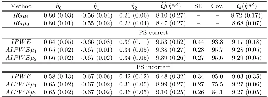
Note that here, in contrast to the first scenario, G_η does not contain gopt. Thus, goptη represents the optimal regime within the class Gη but may not achieve the same perfor-mance as the overall gopt. Via Monte Carlo simulation using 106 replicates, we found that

goptη =I(0.66−0.67X1+ 0.33X2 >0) and E{Y∗(gηopt)}= 9.33 (<9.50), so thatgηopt results in less than a 2% reduction in mean outcome relative to the overall optimal regime.

Table 3.2 shows results for this scenario, where again the genetic algorithm described

pre-viously was used to implement the estimators based on (2.2) and (2.3); results using the grid

search were similar and are shown in Appendix B. The regression estimators based on both incorrect working outcome regression models yield estimated optimal regimes in the class that

are far from achieving the performance of the true optimal regime. In contrast, the proposed

estimators based on both (2.2) and (2.3) exhibit better performance, with a considerable gain in efficiency for those based on AIP W E(η) over that using IP W E(η). Evidently,

augmenta-tion using an incorrect outcome regression model leads to considerable gains over the IPWE regardless of whether or not the propensity score model is correct. Confidence intervals for

E{Y∗(goptη )} when the propensity model was correctly specified achieve the nominal level; not unexpectedly, those based on the AIPWE with misspecified propensity yield poor performance. In Figure 3.2, because the true optimal regime gopt _{is unachievable if we restrict to the} feasible class G_η, we plot the empirical cdfs of the ratios Q(η_bopt)/E{Y∗(goptη )}, which are now different from the ratios Q(ηb

opt_)/E{Y∗_(gopt_{)}. Becauseg}opt

η and gopt lead to overall mean out-comes that differ by less than 2%, these ratios are also informative of the performance of the

estimated regimes relative to the true optimal regime. The figure provides graphical

corrobora-tion of the results in Table 3.2, namely, that the AIPWE may lead to more reliable inference on the optimal regime than the regression estimator or IPWE, exhibiting the desired robustness

to misspecification of one or both models.

3.1.2 Additional Simulation Scenarios

0.80 0.85 0.90 0.95 1.00

0.0

0.2

0.4

0.6

0.8

1.0

PS correct R

Fn(R)

1:RG1 2:RG2 3:IPWE 4:AIPWE1 5:AIPWE2

1 2 3 4 5

0.80 0.85 0.90 0.95 1.00

0.0

0.2

0.4

0.6

0.8

1.0

PS incorrect R

Fn(R)

1:RG2 2:RG1 3:IPWE 4:AIPWE1 5:AIPWE2

1 2 3

4 5

Table 3.2: Results for the second simulation scenario using 1000 Monte Carlo data sets with

n= 500. For the true optimal regime goptη within the classGη, (η0, η1, η2) = (0.66,−0.67,0.33) and E{Y∗(gηopt)}= 9.33. All other quantities are analogous to those in Table 3.1, with µ1 and

µ2 denoting the given estimator using the misspecified models µ1(A, X;β) and µ2(A, X;β), respectively.

Method η_b0 η_b1 η_b2 Qb(η_bopt) SE Cov. Q(η_bopt)

RGµ1 0.80 (0.03) -0.56 (0.04) 0.20 (0.06) 8.10 (0.27) – – 8.72 (0.17))

RGµ2 0.80 (0.01) -0.55 (0.02) 0.23 (0.04) 8.47 (0.27) – – 8.68 (0.07) PS correct

IP W E 0.64 (0.05) -0.66 (0.08) 0.36 (0.11) 9.53 (0.52) 0.44 93.8 9.17 (0.18)

AIP W Eµ1 0.65 (0.02) -0.67 (0.01) 0.34 (0.05) 9.38 (0.27) 0.28 95.7 9.28 (0.05)

AIP W Eµ2 0.66 (0.02) -0.67 (0.02) 0.34 (0.05) 9.39 (0.26) 0.27 95.6 9.29 (0.05)

PS incorrect

IP W E 0.58 (0.13) -0.67 (0.06) 0.42 (0.12) 9.48 (0.32) 0.34 95.0 9.03 (0.35)

AIP W Eµ1 0.65 (0.02) -0.67 (0.02) 0.36 (0.05) 8.99 (0.27) 0.27 75.5 9.27 (0.06)

AIP W Eµ2 0.65 (0.02) -0.67 (0.02) 0.36 (0.05) 9.10 (0.25) 0.26 84.1 9.27 (0.05)

Discrete Covariates Scenario

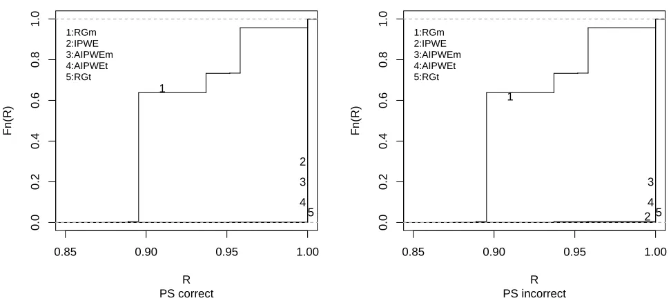
We generated n= 500 observations (Yi, Ai, Xi), i= 1, . . . , n, where Xi = (Xi1, Xi2)T and Xi1 and Xi2 independent with Xi1 Poisson with λ= 2 and Xi2 Bernoulli with success probability 0.5; givenXi,Aiwere Bernoulli with success probability satisfying logit{pr(A= 1|X)}=−0.8+ 0.2X1+ 0.2X2, logit(u)=log{u/(1−u)}; and outcomes were generated asYi =µ(Ai, Xi) +ifor

i standard normal and µ(A, X) = exp{2.0−1.5X12−1.5X2+ 3.0X1X2+A(−1 +X1−X2)}. It is straightforward to deduce that the optimal treatment regime gopt(X) =I(X1 > X2+ 1), a hyperplane in two dimensional space. Via Monte Carlo simulation with 106 replicates, we obtainedE{Y∗(gopt_{)}= 3.71, E{Y}∗_{(0)}= 3.25 and E{Y}∗_{(1)}= 2.51.}

To estimate the optimal regime, we considered the regression estimator and the

estima-tors based on maximizing IP W E(η) in (2.2) and AIP W E(η) in (2.3) in η, respectively, using both correctly and incorrectly specified models µ(A, X;β) and π(X;γ). In particular,

we considered two posited outcome regression models, which we denote as µt(A, X;β) = exp{β0+β1X12+β2X2+β3X1X2+A(β4+β5X1+β6X2)}, corresponding to the correct spec-ification; andµm(A, X;β) =β0+β1X1+β2X2+A(β3+β4X1+β5X2), which is misspecified. We estimated β in each model by least squares. For π(X;γ), we considered the correctly

spec-ified model logit{πt(X;γ)} = γ0+γ1X1 +γ1X2 and was fitted via ML; an incorrect version

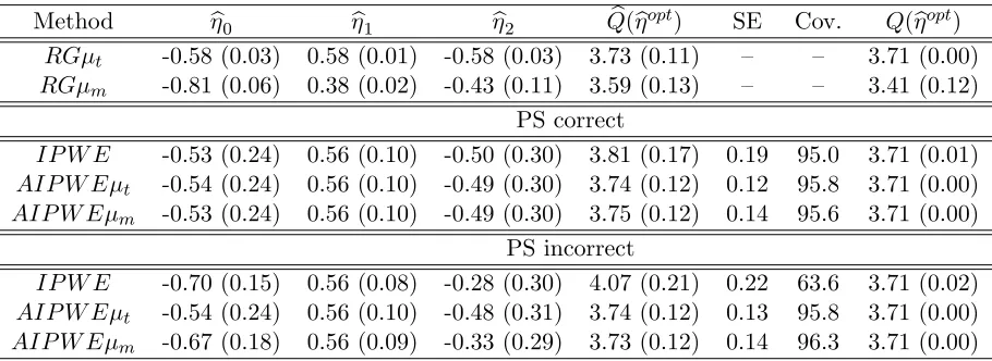
Table 3.3: Results for the discrete covariates simulation scenario using 1000 Monte Carlo data sets with n = 500. For the true optimal regime gopt = gηopt within the class Gη, (η0, η1, η2) = (−0.58,0.58,−0.58) and E{Y∗(gopt)η} = 3.71. All other quantities are analogous to those in Table 3.1.

Method η_b0 η_b1 η_b2 Qb(

b

ηopt) SE Cov. Q(η_bopt)

RGµt -0.58 (0.03) 0.58 (0.01) -0.58 (0.03) 3.73 (0.11) – – 3.71 (0.00)

RGµm -0.81 (0.06) 0.38 (0.02) -0.43 (0.11) 3.59 (0.13) – – 3.41 (0.12) PS correct

IP W E -0.53 (0.24) 0.56 (0.10) -0.50 (0.30) 3.81 (0.17) 0.19 95.0 3.71 (0.01)

AIP W Eµt -0.54 (0.24) 0.56 (0.10) -0.49 (0.30) 3.74 (0.12) 0.12 95.8 3.71 (0.00)

AIP W Eµm -0.53 (0.24) 0.56 (0.10) -0.49 (0.30) 3.75 (0.12) 0.14 95.6 3.71 (0.00)

PS incorrect

IP W E -0.70 (0.15) 0.56 (0.08) -0.28 (0.30) 4.07 (0.21) 0.22 63.6 3.71 (0.02)

AIP W Eµt -0.54 (0.24) 0.56 (0.10) -0.48 (0.31) 3.74 (0.12) 0.13 95.8 3.71 (0.00)

AIP W Eµm -0.67 (0.18) 0.56 (0.09) -0.33 (0.29) 3.73 (0.12) 0.14 96.3 3.71 (0.00)

Table 3.3 and Figure 3.3 show the results for this scenario.

Randomized Trial Scenario

For each data set, we generated n = 500 observations (Yi, Ai, Xi), i = 1,...,n, where Xi = (Xi1, Xi2, Xi3)T with Xi1 and Xi2 independent and uniformly distributed on (−1.5,1.5); Xi3 was Bernoulli with success probability 0.5; givenXi,Ai were Bernoulli with success probability 0.5; and outcomes were generated asYi =µ(Ai, Xi) +i fori standard normal andµ(A, X) = exp{2.0−1.5X₁2−1.5X₂2+3.0X1X2+A(−0.1−X1+X2+0.2X3)}, with correspondinggopt(X) =

I(X2 > X1 −0.2X3 + 0.1), for which Monte Carlo simulation using 106 replicates yielded

E{Y∗(gopt)}= 3.95, E{Y∗(0)}= 3.02 andE{Y∗(1)}= 3.14.

We considered two posited outcome regression models, which we denote as µt(A, X;β) = exp{β0+β1X12+β2X22+β3X1X2+A(β4+β5X1+β6X2+β7X3)}, corresponding to the correct

specification; and µm(A, X;β) = β0+β1X1 +β2X2 +A(β3 +β4X1 +β5X2 +β6X3), which is misspecified. We estimated β in each model by least squares. As this was a randomized study, the propensity score π(X) was estimated directly by the sample proportion assigned to

treatment 1.

0.85 0.90 0.95 1.00

0.0

0.2

0.4

0.6

0.8

1.0

PS correct R

Fn(R)

1:RGm 2:IPWE 3:AIPWEm 4:AIPWEt 5:RGt

1

2 3 4 5

0.85 0.90 0.95 1.00

0.0

0.2

0.4

0.6

0.8

1.0

PS incorrect R

Fn(R)

1:RGm 2:IPWE 3:AIPWEm 4:AIPWEt 5:RGt

1

2 3 4 5

Table 3.4: Results for the randomized trial simulation scenario using 1000 Monte Carlo data sets with n = 500. For the true optimal regimegopt=gηoptwithin the classGη, (η0, η1, η2, η3) = (0.07,−0.70,0.70,0.14) andE{Y∗(goptη )}= 3.95. All other quantities are analogous to those in Table 3.1.

Method ηb0 bη1 bη2 ηb3 Qb(ηb

opt_{) SE Cov. Q(}

b

ηopt)

RGµt -0.07 (0.02) -0.70 (0.01) 0.70 (0.01) 0.14 (0.02) 3.94 (0.15) – – 3.95 (0.00)

RGµm 0.10 (0.29) -0.48 (0.23) 0.47 (0.23) 0.48 (0.35) 3.69 (0.20) – – 3.66 (0.10) PS correct

IP W E -0.07 (0.18) -0.65 (0.12) 0.65 (0.11) 0.12 (0.26) 4.29 (0.24) 0.28 81.9 3.84 (0.08)

AIP W Eµt -0.07 (0.05) -0.69 (0.03) 0.69 (0.03) 0.15 (0.08) 3.96 (0.16) 0.16 95.2 3.94 (0.01)

3.1.3 Simulation Scenarios for Comparison to Marginal Structural Mean Model Approach

We report here on the results of two simulations comparing our proposed methods to the MSMM approach of Robins et al. (2008) and Orellana et al. (2010) in the single decision setting. In both

scenarios below, we used the approach outlined in section 2.3 to implement the MSMM. In the

first scenario, we consider the case where the posited MSMMM(η, τ) is correctly specified; in the second scenario, it is not.

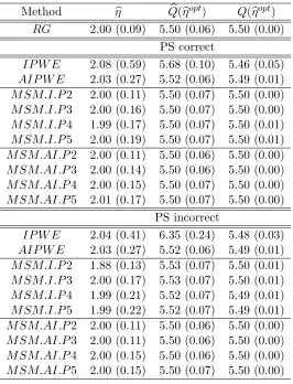
Simulation with Correct MSMM

In this scenario, we generated n = 500 observations (Yi, Ai, Xi), i = 1, . . . , n, where Xi was uniform distributed on (0,4); given Xi, Ai were Bernoulli with success probability satisfying logit{pr(A= 1|X)} = 0.5−0.25X; and outcomes were generated asYi =µ(Ai, Xi) +i fori standard normal andµ(A, X) = 3.0 +X+A(2.0−X), with correspondinggopt(X) =I(X <2). Monte Carlo simulation using 106 replicates yieldedE{Y∗(gopt)}= 5.50,E{Y∗(0)}= 5.00 and

E{Y∗(1)} = 5.00. We considered the class of treatment regimes G_η with elements gη of the

form I(X < η)}, so that gopt ∈ Gη. Thus, for each fixed η, the true Q(η) = E{Y∗(gη)} =

E{µ(1, X)I(X < η) +µ(0, X)I(X ≥η)}=−η2/8 +η/2 + 5.

We considered a correctly specified outcome regression model, which we denote asµ(A, X;β) =

β0+β1X+A(β2+β3X). Forπ(X;γ), we considered both a correctly specified model logit{πt(X;γ)}=

γ0+γ1X, fitted via ML; and an incorrect versionπm(X;γ) =γ0, whereγ0was estimated directly by the sample proportion assigned to treatment 1.

To implement the MSMM approach, we considered models for Q(η) of the form (2.5) with

k0 ranging from 2 to 5. From above, all such models are correct in this scenario. Table 3.5

show the results. Our proposed AIPWE estimator and the MSMM estimators forQ(ηopt) show comparable performance; our IPWE estimator is relatively inefficient and shows similar sample size related bias to that exhibited in the simulations of the main paper. As expected, our

estimators for η are inefficient relative to those from the MSMM approach, owing to the fact

that the MSMM in (2.5) is correctly specified.

The posited MSMMM(η, τ) usually will be an empirical approximation forQ(η) likely not

based on theoretical considerations. Accordingly, we would not expect this model to be correctly

specified in general. We investigate this situation in the next set of simulations.

Simulation With Incorrect MSMM

0.80 0.85 0.90 0.95 1.00

0.0

0.2

0.4

0.6

0.8

1.0

PS correct R

Fn(R)

1:RGm 2:IPWE 3:AIPWEm 4:AIPWEt 5:RGt

1 2 3

4 5

Figure 3.4: Empirical cdfs across 1000 Monte Carlo data sets with n = 500 using correct propensity score (PS) models of the quantities Q(ηb

opt_)/E{Y∗_(ηopt

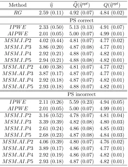
Table 3.5: Results for the correct MSMM simulation scenario using 1000 Monte Carlo data sets with n = 500. For the true optimal regime gopt _{= g}opt

η within the class Gη, η = 2 and

E{Y∗(goptη )} = 5.50. RG represents the regression method using the posited correct outcome regression model; IP W E is our proposed method using 2.2; and AIP W E is our proposed method using 2.3 and the posited correct outcome regression model.M SM.I.P k0 is the MSMM method using (2.6)-(2.7) with polynomial of degree k0. M SM.AI.P k0 is the MSMM method using (2.8)-(2.9) with polynomial of degree k0. The columnηbshows Monte Carlo average

esti-mate, with Monte Carlo standard deviation in parentheses. The column Qb(η_bopt) shows Monte

Carlo average and standard deviation of the estimated values of the true E{Y∗(goptη )}, and

Q(η_bopt) shows the Monte Carlo average and standard deviation of valuesE{Y∗(g_bηopt)}obtained using 106 _{Monte Carlo simulations for each data set.}

Method η_b Qb(

b

ηopt) Q(η_bopt)

RG 2.00 (0.09) 5.50 (0.06) 5.50 (0.00) PS correct

IP W E 2.08 (0.59) 5.68 (0.10) 5.46 (0.05)

AIP W E 2.03 (0.27) 5.52 (0.06) 5.49 (0.01)

M SM.I.P2 2.00 (0.11) 5.50 (0.07) 5.50 (0.00)

M SM.I.P3 2.00 (0.16) 5.50 (0.07) 5.50 (0.00)

M SM.I.P4 1.99 (0.17) 5.50 (0.07) 5.50 (0.01)

M SM.I.P5 2.00 (0.19) 5.50 (0.07) 5.50 (0.01)

M SM.AI.P2 2.00 (0.11) 5.50 (0.06) 5.50 (0.00)

M SM.AI.P3 2.00 (0.14) 5.50 (0.06) 5.50 (0.00)

M SM.AI.P4 2.00 (0.15) 5.50 (0.07) 5.50 (0.00)

M SM.AI.P5 2.01 (0.17) 5.50 (0.07) 5.50 (0.00)

PS incorrect

IP W E 2.04 (0.41) 6.35 (0.24) 5.48 (0.03)

AIP W E 2.03 (0.27) 5.52 (0.06) 5.49 (0.01)

M SM.I.P2 1.88 (0.13) 5.53 (0.07) 5.50 (0.01)

M SM.I.P3 2.00 (0.17) 5.53 (0.07) 5.50 (0.01)

M SM.I.P4 1.99 (0.21) 5.52 (0.07) 5.49 (0.01)

M SM.I.P5 1.99 (0.22) 5.52 (0.07) 5.49 (0.01)

M SM.AI.P2 2.00 (0.11) 5.50 (0.06) 5.50 (0.00)

M SM.AI.P3 2.00 (0.11) 5.50 (0.06) 5.50 (0.00)

M SM.AI.P4 2.00 (0.15) 5.50 (0.06) 5.50 (0.00)