ABSTRACT
KUNDU, PRITHWISH. Tabulated Combustion Model Development For Non-Premixed Flames . (Under the direction of Dr. Alexei Saveliev and Dr. Tarek Echekki.)
©Copyright 2015 by Prithwish Kundu
Tabulated Combustion Model Development For Non-Premixed Flames
by
Prithwish Kundu
A dissertation submitted to the Graduate Faculty of North Carolina State University
in partial fulfillment of the requirements for the Degree of
Doctor of Philosophy
Aerospace Engineering
Raleigh, North Carolina
2015
APPROVED BY:
Dr. Sibendu Som Dr. Yuanjiang Pei
Dr. Kevin Lyons Dr. Tiegang Fang
Dr. Alexei Saveliev
Co-chair of Advisory Committee
Dr. Tarek Echekki
DEDICATION
BIOGRAPHY
ACKNOWLEDGEMENTS
This work would not have been possible without the support of my academic advisors Dr. Tarek Echekki and Dr. Alexei Saveliev. They helped me at the most difficult time of my career. Dr. Echekki’s guidance on the research project was instrumental in the completion of this work. I learnt a lot of turbulent combustion concepts in his MAE 704, advanced combustion course and hope to inherit at least a small fraction of his knowledge in combustion. I would like to thank Dr. Sibendu Som for giving me this opportunity and opening the door to work in collaboration with his team and setting up the project from scratch. The foundation pillar of this project was a result of Dr. Som’s hard work and success over the past 10 years. Dr. Pei’s help in setting up the project and his vast experience had a very positive impact on the work. His constant support was one of the most helpful and comforting factors in this journey. I would also like to thank Dr. Lyons and Dr. Fang for their support as committee members. I would like to thank Zhaoyu Luo, Raju Mandhapati and Mingjie Wang from Convergent Science Inc. for their help with the source codes. I would also like to acknowledge the help from Peter Kelly Senecal and Eric Pomranning for giving us access to the Converge resources. I would also like to thank my MS thesis advisor Dr. William Roberts for introducing me to the interesting world of combustion and getting me started in this field. Last but not the least, I would like to thank Dr. M S Loknath who is no longer with us. He was the first teacher to introduced our class to the field of CFD during my undergraduate days, thanks for inspiring us and believing in us.
throughout my PhD during the dark days, even cooked food for me when I would work late in the lab. They were my family away from home: Deepak, Rahul, Pakkam, Un-kil, Maloo, Anurag, Darshil, Nitish, Sid, Munawira, Prajakta, Soumya, Kushal, Hemal, Pandu, Subbu, Chintan, Sai, Shashank, Sharan, Mukta, Nishant, Naman and Kamal. I could not have survived without their support. I would like to thank all my old and current lab-mates for the help and fun we had: Joe, Brian, Myles, Scott, Richa, Myrrha, Guriqbal, Parth, Shubham, Abhishek, Saini, Shreyas, RC; the Argonne gang: Kaushik, Pei, Quigluan, Anita, Janardhan, Zihan, Roberto, Muhsin, Chao, Moiz and Ruiquin. Annie’s support has been very critical and I cant thank her enough for her help.
TABLE OF CONTENTS
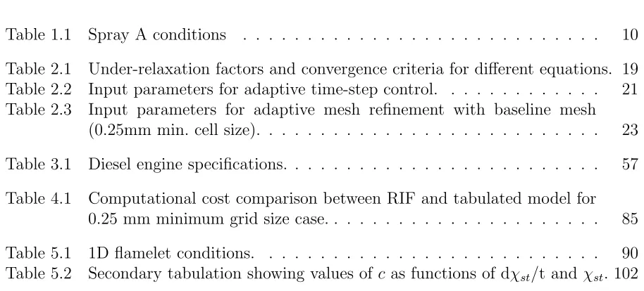
LIST OF TABLES . . . viii
LIST OF FIGURES . . . ix
Chapter 1 INTRODUCTION . . . 1
1.1 Engine Combustion Modeling . . . 1
1.2 Combustion Modeling of Spray Flames . . . 2
1.2.1 Challenges in Combustion Modeling . . . 4
1.2.2 Unsteady Strain Effects . . . 5
1.2.3 Engine Combustion Network Spray A . . . 8
1.2.4 Spray A Experimental Setup . . . 10
1.3 Dissertation Objectives . . . 11
Chapter 2 CFD Model Set Up for Spray Flames . . . 13
2.1 Model Setup in 3D RANS Code . . . 13
2.1.1 Governing Equations . . . 14
2.1.2 Turbulence Model . . . 15
2.1.3 Spray Model . . . 17
2.1.4 Numerical Parameters . . . 19
2.2 Mesh . . . 21
2.3 Reaction Mechanisms . . . 25
2.4 High Performance Computing Resources . . . 26
2.5 Conclusions . . . 27
Chapter 3 The Representative Interactive Flamelet Model . . . 28
3.1 Introduction . . . 28
3.1.1 Governing Equations . . . 29
3.2 Modeling Spray Flames with RIF . . . 32
3.2.1 Non-reacting Cases . . . 32
3.2.2 Grid Convergence . . . 34
3.2.3 Effect of Multiple Flamelets . . . 35
3.2.4 Presumed Form of Scalar PDFs . . . 44
3.2.5 Temperature Sweep . . . 46
3.2.6 Ambient Oxygen Sweep . . . 48
3.2.7 Injection Pressure Sweep . . . 50
3.2.8 Ambient Density Sweep . . . 52
3.2.9 Qualitative Difference Between RIF and Well-Mixed Model . . . . 52
3.3 Diesel Engine Modeling with RIF Model . . . 55
3.3.2 Results with Multiple Flamelets . . . 60
3.3.3 Qualitative Results . . . 62
3.4 Conclusions . . . 65
Chapter 4 Tabulated Combustion Model . . . 67
4.1 Introduction . . . 67
4.2 Chemistry Tabulation . . . 69
4.2.1 Tabulation Structure . . . 69
4.2.2 Turbulence-Chemistry Interactions . . . 71
4.2.3 Multi-Dimensional Table Generation . . . 73
4.3 Tabulated Model Implementation in 3D Code . . . 73
4.3.1 Model Validation . . . 74
4.3.2 Temperature Sweep . . . 76
4.3.3 Injection Pressure Sweep . . . 81
4.3.4 Ambient Oxygen Sweep . . . 81
4.3.5 Computational Cost . . . 84
4.3.6 Differences Between Tabulated Model and RIF . . . 85
4.4 Conclusions . . . 87
Chapter 5 Incorporating Unsteady Effects in Flamelets . . . 89
5.1 Introduction . . . 89
5.2 Evaluation of Unsteady Effects in Flamelets . . . 90
5.2.1 Factors Affecting Unsteady Strain Effects . . . 94
5.3 Equivalent Strain Model . . . 95
5.3.1 Weight Function . . . 97
5.3.2 Model Validation in 1D Code . . . 99
5.3.3 Implementation in the 3D Code . . . 101
5.3.4 Validation of Equivalent Strain model in the 3D Code . . . 103
5.4 Conclusions . . . 106
Chapter 6 Conclusions . . . 111
6.1 Future Work . . . 113
LIST OF TABLES
Table 1.1 Spray A conditions . . . 10
Table 2.1 Under-relaxation factors and convergence criteria for different equations. 19 Table 2.2 Input parameters for adaptive time-step control. . . 21 Table 2.3 Input parameters for adaptive mesh refinement with baseline mesh
(0.25mm min. cell size). . . 23
Table 3.1 Diesel engine specifications. . . 57 Table 4.1 Computational cost comparison between RIF and tabulated model for
0.25 mm minimum grid size case. . . 85
LIST OF FIGURES
Figure 2.1 Schematic showing the spray breakup and evaporation processes. . . 18
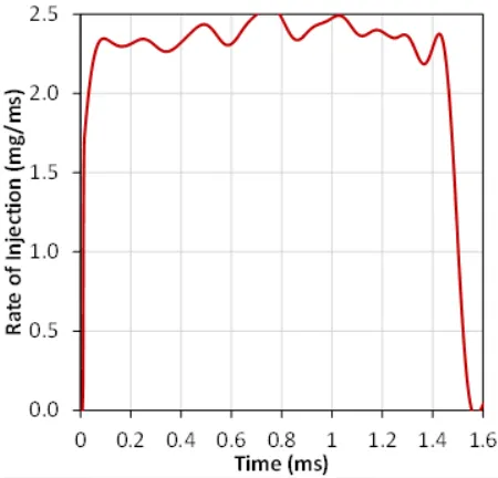
Figure 2.2 Rate of Injection for Spray A at 150 MPa injection pressure. . . 18
Figure 2.3 Adaptive Mesh Refinement: Comparison between (a) coarse mesh (0.5mm smallest grid size) and (b) fine mesh (0.25mm smallest grid size) for Spray A conditions at different time-steps. . . 24
Figure 2.4 0D simulations with 103 and 106 species reaction mechanism for n-dodecane showing ignition delay as a function of temperature at 6 MPa pressure and equivalence ratio of 2. . . 26
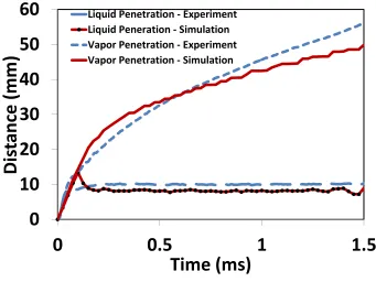
Figure 3.1 Temporal evolution of liquid penetration and vapor penetration for non-reacting Spray A case. . . 33
Figure 3.2 Temporal evolution of lift-off lengths for different grids. . . 35
Figure 3.3 Temporal evolution of lift-off lenghts for multiple flamelets. . . 36
Figure 3.4 Ignition delay and lift-off lengths for different number of flamelets. . . 37
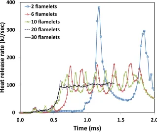
Figure 3.5 Temperature contour plots for cases with different number of flamelets. 38 Figure 3.6 Stoichiometric Scalar dissipation rate evolution for different flamelets. 39 Figure 3.7 Heat Release Rates for multiple flamelets. . . 40
Figure 3.8 Stoichiometric scalar dissipation rate along centre line. . . 41
Figure 3.9 Computational wall clock time for different flamelets. . . 42
Figure 3.10 Lift-off lengths at 1200 K. . . 43
Figure 3.11 Temperature contour comparisons for different presumed PDF func-tions: (a) delta PDF, (b) beta PDF, and (c) Gaussian PDF. . . 45
Figure 3.12 OH contour comparisons for different presumed PDF functions: (a) delta PDF, (b) beta PDF, and (c) Gaussian PDF. . . 45
Figure 3.13 Ignition delay and lift-off lengths for different ambient temperature conditions with delta PDF, beta PDF and Gaussian PDF. . . 47
Figure 3.14 Ignition delay and lift-off lengths for different ambient temperature conditions. . . 49
Figure 3.15 Ignition delay and lift-off lengths for different ambient oxygen concen-trations. . . 51
Figure 3.16 Ignition delay and lift-off lengths for different injection pressures. . . 53
Figure 3.17 Ignition delay and lift-off for different ambient densities. . . 54
Figure 3.18 Qualitative results from RIF and well-mixed model:(a) OH mass frac-tion contour (b) Temperature contour. . . 55
Figure 3.19 Qualitative results from RIF and well-mixed model, temperature con-tour for 13 percent ambient O2 conditions. . . 56
Figure 3.20 Adaptive Meshing for Engine Cases. . . 58
Figure 3.22 Heat Release Rate for Diesel Engine Case. . . 60 Figure 3.23 Pressure Trace for Diesel Engine Case. . . 61 Figure 3.24 Temperature contour plots for single cylinder diesel engine simulations
with single and 80 flamelets at different crank angle degrees. . . 63 Figure 3.25 Temperature contour plots for single cylinder diesel engine simulations
with 1 and 80 flamelets at different crank angle degrees. . . 63 Figure 3.26 CO and NOx mass fraction contour plots for single cylinder diesel
engine simulations with 1 and 80 flamelets. . . 64
Figure 4.1 Schematic of flamelet model. . . 70 Figure 4.2 Temopral evolution of oxygen in flamelet space. . . 72 Figure 4.3 Schematic showing implementation of tabulated model in CFD code. 74 Figure 4.4 Temperature and OH mass fraction predictions from tabulated model. 75 Figure 4.5 Temperature contour comparison between RIF and tabulated model. 77 Figure 4.6 C2H2 and CO mass fraction predctions from RIF and tabulated model. 78 Figure 4.7 Flame temperatures and lift-off lengths for 800K and 900K ambient
temperatures using tabulated combustion model. . . 79 Figure 4.8 Ignition delay and lift-off lengths for Spray A across a range of ambient
temperatures. . . 80 Figure 4.9 Ignition delay and lift-off lengths for Spray A across a range of injection
pressures. . . 82 Figure 4.10 Ignition delay and lift-off lengths for Spray A across a range of oxygen
concentrations. . . 83 Figure 4.11 Computational speed up for different cases with tabulated model. . . 84
Figure 5.1 Unsteady flamelet solver algorithm. . . 92 Figure 5.2 Steady strain flamelet solver algorithm. . . 93 Figure 5.3 ’No history’ (steady strain assumption) flamelet solver algorithm. . . 95 Figure 5.4 History effect on auto-ignition of flamelets under varying scalar
dissi-pation rates for different gradients. . . 96 Figure 5.5 Weight Function. . . 97 Figure 5.6 History effect on auto-ignition of flamelets under varying scalar
dissi-pation rates for different gradients. . . 100 Figure 5.7 Auto-ignition of flamelets for different scalar dissipation rate gradients
and magnitudes. . . 101 Figure 5.8 Block diagram showing implementation of the equivalent strain model
in the 3D code. . . 103 Figure 5.9 Temporal evolution of maximum temperature in domain compared for
RIF, tabulated and equivalent strain model. . . 104 Figure 5.10 Lift-off lengths predicted by RIF model, tabulated model and
Figure 5.11 Ignition delay and lift-off lengths predicted by RIF model, tabulated model and tabulated model with history effects across ambient tem-peratures. . . 108 Figure 5.12 History effect on ignition of Spray A: OH contours from tabulated
model and tabulated model with history effects. . . 109 Figure 5.13 Ignition delay and lift-off lengths predicted by RIF model, tabulated
Chapter 1
INTRODUCTION
1.1
Engine Combustion Modeling
1.2
Combustion Modeling of Spray Flames
1.2.1
Challenges in Combustion Modeling
1.2.2
Unsteady Strain Effects
It has been shown in many experimental and numerical studies that non-premixed flames are subject to unsteady strain effects. These unsteady effects can affect species produc-tion, auto-ignition and extinction. These effects cannot be captured using tabulated mod-els. Tabulated models calculate species mass fractions based on the independent variables of the current time step. These unsteady effects have significant influence on ignition and extinction and need to be systematically evaluated. Moreover, the variables affecting these effects need to be quantified. The dissertation tries to quantify these effects and develops modeling approaches that can consider these effects in tabulated models.
then these high strain rates are not sufficient for the flame to extinguish. Similar results were observed by Brown et al. [18]. Barlow et al. [19] studied the effect of a temporal step change (sudden decrease) of strain on flamelets experimentally as well as numeri-cally using the steady flamelet assumption. The results showed that the steady flamelet assumption over predicted the OH and CO species concentrations. This showed the sig-nificance of the history effects on a flamelet. These studies suggested the importance of unsteady effects in flamelets and the inadequacies of the steady strain assumption to predict flame response under temporally changing SDRs. In this study these unsteady effects will be referred to as the history effects.
used to predict species for a CFDF with oscillating strain and compared with detailed unsteady simulations using GRI 3.0 chemistry for methane. The 2D manifold predictions showed a phase shift with the detailed simulation. A 3D manifold was then created where the chemistry was a function of 3 controlling variables. This manifold was generated by running a number of CFDF problems with varying amplitude and frequencies of strain oscillations. No phase shift was observed between predictions from the 3D FGM manifold and the unsteady results. The work was further extended to extinction limits in [22].
1.2.3
Engine Combustion Network Spray A
This coupled with the physics of turbulent mixing makes it difficult to model and under-stand the auto-ignition and flame stabilization phenomena. Spray A focuses on conditions that involve exhaust gas re-circulation in the low temperature combustion regime. A wide range of parametric variations have been carried that cover a wide range of diesel engine conditions. The modeling setup of Spray A is then discussed in the context of a 3D RANS code. This model set up is then validated against experimental data across a wide range of conditions. Further model development, implementation and validations are based on this Spray A setup.
calculations.
1.2.4
Spray A Experimental Setup
The experimental setup consists of a constant-volume combustion chamber, with either ignition of a premixed fuel-air mixture [25] or preheated compressed air [27] used to achieve the target ambient conditions. Once the desired conditions are reached, the fuel is injected into the constant-volume chamber through a single-hole injector. Some im-portant parameters from the experiments are summarized in Table 1.1. The constant volume combustion chamber is equipped with optical access, which enables a wide range of diagnostic measurements. Liquid penetration length, ignition delay and flame lift-off lengths are measured for different operating conditions. Ignition delay was measured by looking at the pressure rise data and OH chemiluminescence was used to find the lift-off lengths.
Table 1.1: Spray A conditions
Parameter Quantity Baseline case conditions
Fuel n-dodecane n-dodecane
Nozzle outlet diameter 90 microns 90 microns
Discharge coefficient 0.86 0.86
Fuel Injection Pressure 50-150 MPa 150 MPa
Injection Duration 1.5 ms 1.5 ms
Injected fuel mass 3.5 mg 3.5 mg
Ambient gas temperature 800-1200K 900K
Ambient gas density 15.7-22.8 kg/m3 22.8 kg/m3
1.3
Dissertation Objectives
The challenges to turbulent combustion modeling are evaluated in this work. The main objective is to develop models that can address these challenges at lower computational costs. The objectives are summarized as follows:
Evaluate RIF model for turbulent spray flames over a wide range of conditions.
In-vestigate the effect of turbulence-chemistry interactions for high pressure, turbulent spray flames. Determine the effect of number of flamelets and evaluate strategies to determine optimum number of flamelets. Then, evalutate these modeling strategies for a single cylinder diesel engine case.
High fidelity combustion models with large chemistry mechanisms are
computation-ally expensive. The goal is to develop a novel tabulated combustion model capable of incorporating unsteady chemical kinetics with large mechanisms at lower com-putational costs. The main feature of the new modeling technique is to implement a model without the use of a progress variable.
Tabualted models have relatively lower computational cost, however, they cannot
account for unsteady effects. These unsteady effects have mot been evaluated for high pressure spray flame configurations. The quantification of these unsteady terms is important to develop tabulated models that can account for unsteady strain ef-fects. Development of such modeling techniques will lead to high fidelity combustion models that are computationally cheaper and account for more physics than the current models.
the implementation of the Representative Interactive Flamelet model available with the CONVERGE code. The RIF model is validated across a wide range of Spray A conditions and a single cylinder diesel engine. An approach to determine the number of flamelets is developed. The conclusions from the constant volume combustion vessel are found to be consistent with the findings from the single cylinder diesel engine simulations. These results show the implementation of a high fidelity flamelet model capable of solving flamelet histories with the use of online libraries.
Chapter 2
CFD Model Set Up for Spray
Flames
2.1
Model Setup in 3D RANS Code
spray combustion problems. The simulations were run on a high performance computing cluster following best practices established in [34].
2.1.1
Governing Equations
The following governing equations are solved in the CFD code in addition to the com-bustion models which will be discussed in detail. The Reynolds-Averaged Navier-Stokes (RANS) equation framework has been used in this work to model turbulent flows. Con-tinuity and momentum equations for compressible flow are shown in Equations 2.1 and 2.2 respectively where ρ is the density, u is the velocity, P is the pressure and S is the source term in continuity equation.
∂ρ ∂t +
∂ρuj
∂xj
=S (2.1)
∂ρui
∂t +
∂ρuiuj
∂xj
=−∂P
∂xi
+∂σij
∂xj
+Mi (2.2)
The stress tensor is given by
σij =µ
∂ui
∂xj
+∂uj
∂xi
+
µ0− 2 3µ ∂uk ∂xk δij (2.3)
Where µ is the viscosity and δij is the Kronecker delta. u is the velocity, ρ is the
density. M is the source term in momentum equation. The energy equation is given by
∂ρe ∂t +
∂ujρe
∂xj
=P∂uj ∂xj
+σij
∂ui ∂xj + ∂ ∂xj K∂T ∂xj + ∂ ∂xj ρDX m hm ∂Ym ∂xj !
where Y is the mass fraction of specie m, D is the mass diffusion coefficient
The finite-rate chemistry combustion model is implemented by solving transport equa-tions for each specie as shown in Equation 2.5 where ωm is the source term for specie m
and ρm =ρYm. This model does not consider the turbulence-chemistry interactions. The
other combustion models and the ones developed are discussed in detail in the proceeding chapters.
∂ρm
∂t +
∂ρmuj
∂xj = ∂ ∂xj ρDm ∂Ym ∂xj
+ωm (2.5)
2.1.2
Turbulence Model
The implementation of Re-Normalization Group (RNG) k-epsilon model in CONVERGE is discussed in this section. The flow variables are decomposed into an enseble mean and fluctuating term as shown in Equation 2.6.
ui = ¯ui+u
0
i (2.6)
This decomposition when substituted into the Navier-Stokes equations give the com-pressible RANS mass and momentum equations as shown in Equation 2.7 and 2.8.
∂ρ¯
∂t + ∂ρ¯uej
∂xj
= 0 (2.7)
∂ρ¯uei
∂t +
∂ρ¯ugiuj
∂xj
= ∂P¯
∂xi + ∂ ∂xj µ
∂uei
∂xj
+ ∂uej
∂xi
− 2 3µ
∂uek
∂xk δij + ∂ ∂xj
−¯ρug0iu0j
(2.8)
The modeled Reynolds stress for the RNG model is given by 2.9.
τij = 2µtSij −
2 3δij
ρk+µt
∂uei
∂xi
(2.9)
where turbulent viscosity is given by µt=cµρk
2
ε and turbulent kinetic energy (TKE)
as k= 1 2ug
0
iu0i. The strain rate tensor is given by Equation 2.10
Sij =
1 2
∂uei
∂xj
+∂uej
∂xi
(2.10)
Turbulent diffusion and conductivity are given by Equations 2.11 and 2.12 respectively where Sct is the turbulent Shmidt number and Prt is the turbulent Prandtl number.
Dt=
1
Sct
µt (2.11)
Kt =
1
P rt
µtcp (2.12)
The transport equations for turbulent kinetic energy (k) and dissipation of TKE (ε) are given by Equation 2.13 and 2.14 respectively.
∂ρk ∂t +
∂ρuik
∂xi
=τij
∂ui
∂xj
+ ∂
∂xj
µ P rk
∂k ∂xj
−ρε+Ss (2.13)
∂ρε ∂t +
∂ρuiε
∂xi
= ∂
∂xj
µ P rε
∂ε ∂xj
−cε3ρε
∂ui
∂xi
+
cε1
∂ui
∂xj
τij −cε2ρε+csSs
ε
k−ρR (2.14)
R = Cµη
3(1−η/η 0) (1 +βη3)
ε2
k (2.15)
η= k
ε |Sij | (2.16)
The modeling constants for the RNG turbulence model for the spray flame simulations in this study were set as Cµ= 0.0845, cε1=1.42, cε2 = 1.68, cε3 =−1.0 andβ = 0.012.
2.1.3
Spray Model
Injection of high pressure liquid fuel sprays in a turbulent atmosphere is modeled in the CONVERGE code . A number of factors affect spray physics and evaporation processes of the liquid fuel. This further influences the fuel air mixing process. The modeling of spray has a direct impact on auto-ignition, flame stabilization and species formation processes. The Lagrangian-Eulerian approach is used to model sprays in CONVERGE where the liquid phase is modeled as Lagrangian particles. The schematic in Figure 2.1 shows the different process that need to be modeled for any given spray combustion problem. The fuel spray coming out of the nozzle will be characterized by the radius of the droplets coming out of the nozzle. This is modeled by the primary breakup model. These liquid spray droplets further breakup into smaller droplets depending on a number of factors including aerodynamic drag, instabilities and shape of the droplet. This is modeled using a secondary breakup model. The collision between these droplets can have a significant impact on sprays. These liquid droplets are also subject to evaporation and eventual mixing with the oxidizer. All these coupled process require an accurate spray model.
Figure 2.1: Schematic showing the spray breakup and evaporation processes.
fuel ndodecane was used for this study. The liquid properties are supplied to the code in the form of a ’liquid.dat’ text file. The rate of injection (ROI) was implemented for the Spray A case from available experimental data and is shown in Figure 2.2.
Figure 2.2: Rate of Injection for Spray A at 150 MPa injection pressure.
Table 2.1: Under-relaxation factors and convergence criteria for different equations.
Equation Under-relaxation Convergence criteria
Pressure 1.6 10-7
Momentum 1.0 10-4
Energy 1.0 10-4
Mass 1.0 10-4
Species 1.0 10-4
Passive 1.0 10-4
TKE 0.7 10-3
Epsilon 0.7 10-3
secondary breakup process. The no time counter algorithm [37] was adopted to account for droplet collisions. Frossling correlation was used for modeling droplet evaporation [38]. A dynamic drag model [39] and a turbulent dispersion model were used to model droplet drag and dispersion.
2.1.4
Numerical Parameters
The finite volume differencing scheme was used in the CONVERGE code to solve the governing equations with a transient implicit solver. The Pressure Implicit with Splitting of Operators (PISO) scheme was used for the pressure-velocity coupling. Under-relaxation was used to aid convergence for the transport equations. The convergence criteria is calculated based on a normalized error for each equation. The under-relaxation factors and convergence criteria used in this study are summarized for different equations in Table 2.1.
physics, species production and heat release. The CFL number (u∆t
∆x), Mach CFL number
(c∆∆xt2) and diffusive CFL number (v
∆t
∆x) are used to control the time-stepping in
CON-VERGE. Here u is the velocity, cis the speed of sound and v is the viscosity. Maximum limits are set for each of these CFL numbers along with an initial time step. After each iteration the CONVERGE code tries to increase the current time-step by 25 percent. If the convergence criteria mentioned is not acheieved with the time-step or if it exceeds the CFL number limits then the time-step is reduced. For the spray simulation cases discussed in this study the these CFL number limits and convergence criteria were de-termined based on parametric studies. The maximum value of CFL number allowed in the simulation was restricted to 0.75.
When the spray model is active then the maximum time step is calculated by Equation 2.17 where ∆xis the grid size andmspray is an input parameter from the user which limits
the maximum number of cells a parcel can travels in the given time step. Similarly, other parameters are used to control time stepping based on evaporation and temperature rise in a given cell.
dtspray =min
∆x parcelv
×mspray (2.17)
whereparcelv is the velocity of a parcel the given cell. If droplet evaporation is active in
a fluid domain then the maximum time step is given by Equation 2.18 where Mc is the
total mass of the cell and Mevap is the mass evaporated from the previous time step, and
dt0 is the previous time step. The user input parametermevapthus controls the maximum
allowable evaporated mass in a single time step. Similarly, Equation 2.19 restricts the time step based on temperature rise in each cell where the input parameter is mchem. A
the input parameters for time step control used for the Spray A simulations.
dt evap=dt0×min
Mc
Mevap
×mevap (2.18)
dt chem=dt0×min
T
∆T
×mchem (2.19)
Table 2.2: Input parameters for adaptive time-step control.
Parameter Value
mspray 0.5
mevap 0.5
mchem 0.5
Initial time-step 5e-7 s Minimum time-step 1e-8 s Maximum time-step 1e-6 s
2.2
Mesh
move in space. As a result a large subsection of the mesh needs to be refined. The entire procedure would need to be repeated iteratively based on the solution to arrive at a grid independent solution. This is a brute force approach and in order to demonstrate grid convergence a very large mesh needs to be generated and solved.
Unsteady engine combustion simulations involve spray injection events coupled with moving boundaries. A fine mesh is required only for regions near the spray and a coarse mesh would suffice for the other regions. Fuel air mixing layers that are formed along the stoichiometric regions exhibit the most chemically reactive regions for non-premixed combustion. It is important to have higher mesh resolution in these regions to resolve the chemistry and flow accurately. Adaptive meshing is well suited for such problems and has a robust implementation in Converge for complex as well as moving geometries. The mesh refinement is changed at every time step depending on the solution at each time step as shown in Figure 2.3. In these plots the computational grids are in 3 dimension but the comparisons are made between the slices of x−y plane along the center-line of the spray. The upper half of the domain represents the coarse mesh. The base grid size (dxbase) is the default size of the initial grid generated over the entire domain. This is
set to 4 mm for the baseline mesh. Fixed embedding is a feature that allows the user to refine the grid selectively at certain places. In spray cases usually the region near the nozzle is refined using fixed embedding. The input parameter embedscale determines the
size (dxembed) of mesh near the embedded region and is given by Equation 2.20.
dxembed =dxbase×2−embedscale (2.20)
ms higher resolution grids are generated in the flame region.
The AMR algorithm in CONVERGE adds higher grid resolution at regions where the gradients of specified variables are highest. In this study the AMR was based on velocity and temperature fields. This combination can capture the spray as well as the fuel air mixing regions accurately. The input parameters amrembed vel scale and amrembed temp scale
are used to control the minimum cell sizes generated in regions of high gradients. The mesh size is given by Equation 2.21
dxembed =dxbase×2−amrembed vel scale (2.21)
For the baseline case these values are summarized in Table 2.3. These values will lead to a minimum cell size of 0.25 mm. For running a finer mesh for the same problem only the base grid size is changed. Thus, a base grid size of 2 mm will lead to a minimum grid size of 0.125 mm and 8 mm base grid size will lead to a mesh with smallest grid size of 0.5 mm. These grids are generated at runtime and a new mesh is generated at every time step based on the AMR settings and the solution of the problem.
Table 2.3: Input parameters for adaptive mesh refinement with baseline mesh (0.25mm min. cell size).
AMR Parameter Value
Base grid 4 mm
Nozzle Embed Scale 4
Velocity AMR Embed Scale 4 Temperature AMR Embed Scale 4
2.3
Reaction Mechanisms
Figure 2.4: 0D simulations with 103 and 106 species reaction mechanism for n-dodecane showing ignition delay as a function of temperature at 6 MPa pressure and equivalence ratio of 2.
2.4
High Performance Computing Resources
Each node has 64 GB of Random Access Memory which is shared between 16 proces-sors. The memory available for each node is an important factor especially for tabulated combustion models and for large meshes. The tabulation and cell data are stored in memory during runtime. The Message Passing Interface implementation creates a copy of the arrays for each processor and stores them in the RAM for fast access. This can lead to memory issues for runs with large meshes. Codes were developed considering this memory bottleneck.
The ’Fusion’ cluster is a relatively small machine with a peak performance of 30 teraflops, 320 nodes with 8 processors per node with Infiniband QDR interconnect. Each node shares 36 GB of RAM. This cluster was used to run the Spray A cases with 4 nodes i.e. 32 processors in parallel.
2.5
Conclusions
Chapter 3
The Representative Interactive
Flamelet Model
3.1
Introduction
RNG turbulence model is used in conjunction with a grid-converged discrete phase model for the liquid phase. The minimum number of flamelets required is determined to suf-ficiently represent the large variation of stoichiometric scalar dissipation rates in the domain. Different forms of the presumed scalar probability density functions (PDFs) were also examined. The modeling results are then compared with the experimental data at different ambient temperatures, ambient O2 concentrations, ambient densities, and injection pressures. The effects of different chemical kinetic mechanisms (103-species and 106-species skeletal mechanisms) are also studied to further understand the performance of the model. Overall, the RIF model is observed to capture the measured ignition delay and flame lift-off length very well, especially under certain conditions characterized by low ambient temperatures, densities, and oxygen concentrations. The need for initializing multiple flamelets is highlighted in order to obtain simulation results devoid of model-ing artifacts. Overall, the efficacy of usmodel-ing an advanced turbulent combustion model is demonstrated. The same modeling framework is then applied towards modeling a single cylinder diesel engine. Parametric variations show exactly the same type of trends that were observed with the Spray A cases and the simulation results match well with the reported experimental data.
3.1.1
Governing Equations
The RIF model was proposed and derived by Pitsch et. al. [45], which was based on the laminar flamelet concept by Peters [46] and [47]. The RIF combustion model calculates the species mass fraction based on the knowledge of Favre averaged mixture fraction (Ze)
and mixture fraction variance gZ”2 in the flow field. Therefore, two additional transport
∂( ¯ρZe)
∂t +
∂( ¯ρuelZe)
∂xl
= ∂( ¯ρugl
00Z00)
∂xl
(3.1)
where
g
ul00Z00=−Dt
∂Z˜ ∂xl
(3.2)
∂(ρgZ”2)
∂t +
∂(ρuelZg”2)
∂xl
=−∂(ρug
00
lZ”2)
∂xl
−2(ρug00lZ”)
∂Ze
∂xl
−ρχe (3.3)
The scalar dissipation rate is modeled as χe=cxεkgZ”2 where cx is a mixing constant,
k is the turbulent kinetic energy and ε is the dissipation rate obtained from the turbu-lence model. The value of cx was set equal to 2 for all cases. The flamelet equations 3.4
and 3.5 were derived from the species conservation equation by applying a coordinate transformation to the mixture fraction (Z) space [46].
ρ∂Yi ∂t =ρ
χ
2
∂2Y
i
∂Z2 + ˙ωi (3.4)
ρ∂T ∂t −ρ
χ
2
∂2T
∂Z2 −ρ
χ
2Cp
XCpi
Lei ∂Yi ∂Z + ∂Cpi ∂Z ∂T ∂Z = 1 Cp ∂P ∂t − X ˙
ωihi
(3.5)
In order to solve these set of partial differential equations 3.4 and 3.5, the scalar dissipation rate χ should be converted from a function of physical space to a function of mixture fraction. The following equation 3.6 derived in [46] was used to perform the transformation:
χ(Z) = χcst
f(Z)
f(Zst)
where
f(Z) = exp[−2(erf c−1(2Z))] (3.7)
f
χst is the domain averaged scalar dissipation rate conditional over the stoichiometric
mixture fraction and erfc is the error function. In order to construct the flamelet library for the entire CFD domain, the average value is calculated using Equation 3.8
c
χst =
R
vρχfst
3/2
e
P(Zst)
R
vρχfst
1/2
e
P(Zst)
(3.8)
where
f
χst =χe
f(Zst)
R1
0 f(Z)P(Z)dZ
(3.9)
v is the volume of the entire computational domain and P() is the probability density function (PDF). Solving the flamelet equations 3.4 and 3.5 gives the species mass fraction
Y i as a function of Z. A beta PDF distribution of the mixture fraction as shown in Equation 3.10 is assumed to calculate the mass fraction Yi in each cell with Equation
3.11. The presumed shape of beta PDF,P(Z;x, t), was also used in the previous equation 3.8.
P(Z;x, t) = Ze
α−1(1−
e
Z)β−1
Γ(α)Γ(β) Γ(α+β) (3.10)
e
Yi(x, t) =
Z 1
0
Yi(Z, t)P(Z;x, t)dZ (3.11)
which were solved for each flamelet generated:
∂( ¯ρZel)
∂t +
∂( ¯ρuelZel)
∂xl
=−∂( ¯ρug ”
lZl”)
∂(xl)
(3.12)
These markers must also satisfy 3.13
e
Z =
n
X
1
Zl (3.13)
where n= number of flamelets The averaged value of stoichiometric scalar dissipation rate for each flamelet is calculated as:
c
χst(l) = χcst = R
v
f
Zl
Zρχfst
3/2
e
P(Zst)
R
v
f
Zl
Zρχfst
1/2
e
P(Zst)
(3.14)
3.2
Modeling Spray Flames with RIF
The focus of this study is the reacting cases at different ambient conditions, including variations of ambient temperature, ambient oxygen concentration, injection pressure, and ambient density. The grid convergences for the RIF model was first studied, followed by the selection of number of flamelets. After establishing the baseline setup, comprehensive studies of reacting cases are presented.
3.2.1
Non-reacting Cases
am-0
10
20
30
40
50
60
0
0.5
1
1.5
D
is
ta
n
ce
(m
m
)
Time (ms)
Liquid Penetration - Experiment Liquid Peneration - Simulation Vapor Penetration - Experiment Vapor Penetration - Simulation
Figure 3.1: Temporal evolution of liquid penetration and vapor penetration for non-reacting Spray A case.
bient temperature, 22.8 kg/m3 ambient density with 150 MPa injection was simulated in the CONEVRGE code for an injection duration of 1.5 ms. Liquid penetration is defined as the axial location from the nozzle that encompasses 97 percent of the injected mass at any given time instant. Vapor penetration is defined as the farthest downstream location of 0.05 percent fuel mass fraction contour.
shows a similar trend and the predictions are close to the experimental values with slight under-prediction. Initially the vapor penetration increases rapidly and then increase at a lower rate. This trend is also captured by the simulation. The simulations initially over-predict the vapor pentration and after 0.5 ms of injection show slight over-over-prediction. The spray model captures the spray break-up and mixing process for the Spray A setup.
3.2.2
Grid Convergence
Three meshes with different values of minimum grid size i.e., 0.5 mm, 0.25 mm and 0.125 mm were studied to assess the grid convergence for the RIF combustion model. These minimum grid sizes were obtained from a base mesh size of 1 mm together with different levels of AMR and embedding. This resulted in a peak cell count of about 630,000 for the finest resolution of 0.125 mm at 1.5 ms. The ignition delay and flame lift-off length are the metrics to evaluate the results from different meshes. The ignition delay was calculated based on the maximum temperature in the domain and defined as the time from start of injection (SOI) to the instant of the maximum temperature rise. The lift-off length in experiments was defined based on OH chemiluminescence; however, since OH* was absent from the simulations, the lift-off length was defined as the distance from the injector to the 14 percent maximum ground state OH at steady state. These two definitions are the recommendations from ECN2 workshop (Engine Combustion Network (2013) [1]).
0 5 10 15 20 25 30 35 40
0.3 0.8 1.3
Li ft -o ff l e n g th ( m m ) Time (ms) RIF (0.125mm) RIF (0.25mm) RIF (0.5 mm) Experiment
Figure 3.2: Temporal evolution of lift-off lengths for different grids.
mesh considering the balance of accuracy and computational cost. One may argue the difference for the RIF results at the earlier timing is relatively large between the mesh size 0.25 mm and 0.125 mm. The 0.25 mm mesh was run on This is not going to affect the lift-off length predictions significantly since the lift-off length is an average value over quasi-steady state where the difference for these two meshes is rather small (1 mm). Based on these results the 0.25 mm mesh is chosen as the baseline for calculations.
3.2.3
Effect of Multiple Flamelets
As discussed earlier, one of the shortcomings of the RIF model is that the domain averaged scalar dissipation rateχst cannot capture the effects of the varying scalar dissipation rate
10 15 20 25 30 35
0.5 0.7 0.9 1.1 1.3 1.5
Li ft -o ff l e n g th ( m m ) Time (ms)
Experiment 2 flamelets
6 flamelets 10 flamelets
20 flamelets
Figure 3.3: Temporal evolution of lift-off lenghts for multiple flamelets.
better account for the variation of χst on the RIF model the simulations were run with
19 20 21 22 23 24 0 0.2 0.4 0.6 0.8 1 1.2 1.4 1.6 1.8
0 20 40 60
Li ft -o ff l e n g th ( m m ) Ig n it io n d e la y ( m s)
Number of flamelets
Ignition delay LOL
Figure 3.4: Ignition delay and lift-off lengths for different number of flamelets.
The qualitative results for auto-ignition and flame stabilization for different flamelets are shown in Figure 3.5. It is observed that the single flamelet case ignites at 1.6 ms and does not predict any lift-off behaviour. The 20 and 60 flamelet cases predict identical contours and there is no difference in the qualitative results as well.
1.5 ms 1.6 ms 1.7 ms 1.8 ms 1.9 ms
0.7 ms 0.8 ms 0.9 ms 1.0 ms 1.1 ms
0.6 ms 0.7 ms 0.8 ms 0.9 ms 1.0 ms
0.6 ms 0.7 ms 0.8 ms 0.9 ms 1.0 ms
Figure 3.6: Stoichiometric Scalar dissipation rate evolution for different flamelets.
rate. This occurs successively for each individual flamelet.
This oscillatory behaviour of flame lift-off length (Figure 3.3) can be explained from Figure 3.7, which shows the predictions of heat release rate for different number of flamelets with the RIF model. The heat release rate with 2 flamelets increases after the ignition delay and has 2 bumps. With increase in the number of flamelets the ampli-tude of the oscillations decreases and the frequency goes on increasing with time. Finally, when the number of flamelets is sufficient, the oscillations die down and a steady heat release curve is observed.
0 100 200 300 400
0.0 0.5 1.0 1.5 2.0
H
e
a
t
re
le
a
se
r
a
te
(
k
J/
se
c)
Time (ms)
2 flamelets6 flamelets 10 flamelets 20 flamelets 30 flamelets
0
0.5
1
1.5
2
2.5
3
0
10
20
30
40
lo
g
10(χ
st)
(s
e
c
-1
)
Axial distance (mm)
900K ambient temperature
1200K ambient temperature 1200 K flame stabilization point
900 K flame stabilization point
Figure 3.8: Stoichiometric scalar dissipation rate along centre line.
the axial distance from the noxxle.
80 100
6 7 10 20
T
im
e
(
h
rs
)
Number of flamelets
Figure 3.9: Computational wall clock time for different flamelets.
number of flamelets will result in the resolution of this issue and the fuel packets will ignite more accurately in small amounts depending on local conditions.
The above paragraph clearly demonstrates the need for the RIF model to have a sufficient number of flamelets to account for the large variation of the scalar dissipation rate. In Figure 3.4 the lift-off lengths and ignition delays from 60, 30 and 20 flamelets are almost identical, which indicates that 20 flamelets are sufficient for the baseline RIF cases at 900 K ambient condition. However, Figure 3.4 suggests that 30 flamelets provide a better estimate for the heat release rate. Since our focus is on the predictions of lift-off length and ignition delay in this study, 20 flamelets were adopted for the baseline case. Increasing the number of flamelets results in higher computational cost as shown in Figure 3.9. These simulations were run for the same grids with different number of flamelets on 32 processors.
0 4 8 12 16
0 0.5 1 1.5
Li
ft
-o
ff
l
e
n
g
th
(
m
m
)
Time (ms)
20 flamelets 40 flamelets
Figure 3.10: Lift-off lengths at 1200 K.
under some other conditions show that this estimation is not sufficient. A higher ambi-ent temperature of 1200 K with 1.5 ms duration of injection was simulated with 20 and 40 flamelets as shown in Figure 3.10. One can notice from Figure 3.10 that the lift-off length has oscillatory behaviour with 20 flamelets. This was not observed for the 900 K baseline case with the same number of flamelets. The reason is that the 1200 K case has a shorter lift-off length and a further upstream lift-off location. Thus, the value of χst
around stabilization location is much higher, as presented in Figure 3.8. This indicates that higher χst around the flame stabilization location would require more flamelets to
account for the larger variation ofχst. It is also interesting to note thatχst does not vary
3.2.4
Presumed Form of Scalar PDFs
A presumed form of scalar PDFs was used to calculate the species mass fraction in each cell with the solution from the flamelet equations. This PDF describes the statistical variances occurring in the turbulent flow. Typically beta PDFs are used for turbulent combustion problems. The role played by the form of presumed PDF is studied in detail in this section. Three different schemes were investigated viz. delta, beta and Gaussian PDF. In order to implement a delta PDF the following procedure was followed. The flamelet equations were solved for each flamelet to yield the species mass fractions as functions of Z. The mixture fraction is known for each cell in the CFD domain. This mean value of Z was mapped directly to the flamelet solution to calculate the species mass fraction. This process eliminates the role of the mixture fraction variance and effect of turbulent fluctuations and is same as having a delta PDF.
Figure 3.11 and Figure 3.12 show the qualitative differences between the results ob-tained by delta, beta and Gaussian PDFs. These simulations were set up with the 103 species mechanism and 20 flamelets. The delta PDF which neglects the variances and the integration process predicts a higher temperature and also a higher gradient in OH mass fraction. The peak values of OH are also higher. It can be observed in Figure 3.11(b) that the beta PDF integration results in reduction of temperature and smearing of the gradients. A similar trend is also observed with the OH distribution with beta PDF in Figure 3.12(b) . The beta PDF integration tends to smear the gradients and also results in a reduction of peak values of temperature and OH species mass fraction.
Figure 3.11: Temperature contour comparisons for different presumed PDF functions: (a) delta PDF, (b) beta PDF, and (c) Gaussian PDF.
0.55ms and that from Gaussian PDF was 0.575ms. The experimental value reported was 0.44 msec. However, the Gaussian PDF predicts higher values of OH with a thin region of high concentration of OH as shown in Figure 3.13. Overall, both the PDF integration schemes were able to capture the ignition delays and lift-off lengths. The beta PDF was used for the rest of the study.
Figure 3.13 shows quantitative comparisons of the different PDF integration methods across a sweep of temperatures. Overall, it is observed that the beta PDF as well as Gaussian PDF predict very similar ignition delays; however, the predictions of lift-off lengths from the Gaussian PDF are slightly closer to the experimental values.
3.2.5
Temperature Sweep
these ambient conditions. Similar over-predictions were also observed for the 103 species mechanism except that similar or better predictions were obtained at the higher ambient temperatures of 1000 and 1100 K for the well-mixed model. Comparing the two mecha-nisms for the well-mixed model, one may notice similar predictions for the lower ambient temperature conditions and much better estimations for the 103 species mechanism at the higher ambient temperature conditions. However, this is not observed for the RIF model which predicts similar ignition delays across the ambient temperature conditions considered here.
For the two mechanisms considered, the predictions from the RIF model for lift-off are much better than those of well-mixed model at the lower ambient conditions. Predictions are quite similar for the higher ambient temperature conditions for the 106 species mechanism for the two combustion models. It is interesting to note that the RIF model is less sensitive to the reaction mechanisms used.
3.2.6
Ambient Oxygen Sweep
0
0.2
0.4
0.6
0.8
1
1.2
1.4
1.6
1.8
800
900
1000
1100
Ig
n
it
io
n
d
e
la
y
(
m
s)
Ambient temperature (K)
0
5
10
15
20
25
30
35
40
45
800
900
1000
1100
Li
ft
-o
ff
l
e
n
g
th
(
m
m
)
Ambient temperature (K)
Experiment
Well-mixed, 106 species RIF, 106 species Well-mixed, 103 species RIF, 103 species
predicts the ignition delays significantly better than the well-mixed model for different ambient oxygen concentrations for both the mechanisms. It is noted that the predic-tions at 21 percent oxygen condition are very accurate for both mechanisms. However, at lower ambient oxygen concentrations simulations with both RIF and well-mixed models were found to over-predict ignition delays. The values predicted by the RIF model were significantly better than the well-mixed model.
Lift-off length calculations are also presented in Figure 3.15. The results from both mechanisms over-predict the sensitivity with respect to different ambient oxygen con-ditions for the well-mixed model although relatively good estimations were found for the 21 percent oxygen condition. However, the RIF model predicts better sensitivity for both mechanisms with more accurate estimations at lower oxygen concentration of 13 percent and some over predictions at 15 and 21 percent ambient oxygen conditions. The less sensitivity to the chemistry mechanisms was again observed for the ambient oxygen conditions studied here.
3.2.7
Injection Pressure Sweep
0
0.2
0.4
0.6
0.8
1
1.2
1.4
1.6
1.8
13
15
17
19
21
Ig
n
it
io
n
d
e
la
y
(
m
s)
Ambient oxygen (%)
0
5
10
15
20
25
30
35
40
13
15
17
19
21
Li
ft
-o
ff
l
e
n
g
th
(
m
m
)
Ambient oxygen (%)
ExperimentWell-mixed, 106 species RIF, 106 species Well-mixed,103 species RIF, 103 species
for all injection pressures for both mechanisms. Similar predictions of lift-off lengths are reported, the RIF model predicts correct sensitivity with respect to the variation of injection pressure and more accurate results compared to the experiments for both mechanisms. Again, at different injection pressures over-prediction of the sensitivity to oxygen concentration was observed for the well-mixed model. Consistent with previous findings, the RIF model is less sensitive to the reaction mechanisms used for the conditions considered in this section.
3.2.8
Ambient Density Sweep
The effect of change in ambient density (from baseline condition of 22.8 kg/m3 to 15.7 kg/m3) at 900 K is studied in this section. The predictions of ignition delay and lift-off length are reported in Figure 3.17 and overall similar observations were found. It can be seen that all the simulations over-predict the measurements with RIF better capturing the sensitivity with respect to the variation of ambient density than the well-mixed model. For the lift-off length predictions reported, the RIF model predicts better sensitivity and more accurate results than the well-mixed model compared to the measurements. Less sensitivity of the RIF model to the chemistry mechanism is found again for the conditions studied.
0
0.2
0.4
0.6
0.8
1
50
70
90
110
130
150
Ig
n
it
io
n
d
e
la
y
(
m
s)
Injection pressure (MPa)
0
5
10
15
20
25
30
50
70
90
110
130
150
Li
ft
-o
ff
l
e
n
g
th
(
m
m
)
Injection pressure (MPa)
ExperimentalWell-mixed, 106 species
RIF, 106 species
Well-mixed, 103 species
RIF, 103 species
0
1
2
3
4
5
12
25
Ig
n
it
io
n
d
e
la
y
(
m
s)
Ambient density (kg/m
3)
10
30
50
70
90
12
25
Li
ft
-o
ff
l
e
n
g
th
(
m
m
)
Ambient density (kg/m
3)
ExperimentWell-mixed, 106 species RIF, 106 species
Well-mixed, 103 species RIF, 103 species
Figure 3.18: Qualitative results from RIF and well-mixed model:(a) OH mass fraction contour (b) Temperature contour.
The well-mixed model predicts higher temperatures and OH as compared to the RIF model. The flame structure is also different compared to RIF. The well-mixed model predicts a horse-shoe shaped OH contour with higher gradients. The RIF model on the other hand predicts smeared OH and temperature profiles. The lift-off length predicted by the RIF model is lower compared to that predicted by the well mixed model. Similar comparison at the 13 percent ambient oxygen concentration is shown in Figure 3.19. The RIF model predicts higher temperatures and lift-off lengths. Well-mixed model predicts higher gradients in temperature and the RIF model predicts a smeared profile. Also the RIF model tends to predict a broader flame.
3.3
Diesel Engine Modeling with RIF Model
number of flamelets was investigated using the same method discussed in the previous section.
The experimental setup consisted of a single cylinder turbocharged research engine. The Caterpillar Hydraulic Electronic Unit Injector (HEUI) 315B injector with 6 holes was used in this engine. More details regarding the injector nozzle geometry can be found in [48]. The other engine specifications are listed in Table 3.1. The engine speed was fixed at a constant value of 1500 rpm. The oil rail pressure in the HEUI injection system was set at 170 bar which corresponds to a peak injection pressure of 1122 bar. The cylinder pressure was measured using a piezoelectric water cooled pressure transducer.
Table 3.1: Diesel engine specifications.
Description
Value
Engine Model Caterpillar 3410E
Bore 137.2 mm
Stroke 165.1 mm
Displacement 2.44 L
Compression Ratio 16.278:1
Combustion Air System Simulated turbocharger and air-to-air aftercooler Combustion air system HEUI 315B, six-hole tip
3.3.1
Computational Model
Figure 3.21: Single cylinder engine geometry with sector mesh.
0 20 40 60 80 100 120 140 160
-10 0 10 20
H e a t re le a se r a te ( J/ C A ) Crank angle(deg) 1 flamelet 20 flamelets 40 flamelets 64 flamelets 80 flamelets
Figure 3.22: Heat Release Rate for Diesel Engine Case.
3.3.2
Results with Multiple Flamelets
6.8
7.0
7.2
7.4
7.6
7.8
8.0
-7
-2
3
8
13
18
P
re
ss
u
re
t
ra
ce
(M
P
a
)
Crank angle(deg)
Experiment 1 flamelet 20 flamelets 40 flamelets 64 flamelets 80 flamelets
Figure 3.23: Pressure Trace for Diesel Engine Case.
3.3.3
Qualitative Results
The effect of number of flamelets on engine simulations with respect to pollutant forma-tion and flame lift-off are discussed in this secforma-tion. Figure 3.24 shows the temperature contour plots from Top Dead Centre (TDC) to 50 degrees after TDC. The spray injection starts at -7 crank angle degrees (CAD). An ignited flame is seen at TDC for both the cases before the spray plume has hit the bottom of the engine bowl. The flame shape predicted by the 80 flamelet case differs from the single flamelet case. The single flamelet case predicts high temperature regions in the near nozzle region. A lifted flame structure is predicted by the RIF model with 80 flamelets. Figure 3.25 shows the OH contours at 10 CAD after TDC along with the lift-off iso-contour. It clearly shows that the single flamelet case does not predict a lifted flame. A single flamelet accounts for the entire chemistry of the combustion chamber. When this flamelet reaches an ignited state any fuel in the computational domain will ignite. With the presence of multiple flamelets each flamelet will account for a certain portion of the fuel and ignite independently as per the local scalar dissipation rate conditions. The ECN Spray A cases also showed that single flamelet simulations do not predict lifted flames. These factors influence prediction of pollutants.
Figure 3.24: Temperature contour plots for single cylinder diesel engine simulations with single and 80 flamelets at different crank angle degrees.
3.4
Conclusions
The RIF model with multiple flamelets was used to investigate the effect of turbulent chemistry interactions in spray flames under diesel engine conditions. The model with 2 different reaction mechanisms were validated against the experimental data from Spray A across a wide range of conditions. The RIF model was able to capture auto-ignition and flame lift-off across a wide range of conditions. The need for multiple flamelets to account for large spatial variations in scalar dissipation rate was demonstrated and a detailed analysis on the effect of number of flamelets on the results was presented. The importance of a RIF calculation to demonstrate the convergence with respect to the number of flamelets is highlighted and the minimum number of flamelets required was studied to accurately predict the ignition delay, lift-off length, and heat release rates under different ambient conditions. The model was applied to a single cylinder diesel engine and the results closely matched the experimental pressure trace. The main conclusions are noted below:
1. Sufficient numbers of flamelets are needed to account for the large variation of scalar dissipation rate under different conditions considered in the study. Heat release rates can be used as a metric to verify the sufficiency of flamelets. The same pattern was observed for the constant volume spray flame as well as the single cylinder diesel engine. 2. The RIF model predicts a wider and more distributed flame structure with lower temperatures and OH concentrations than the well-mixed model.
3. Quantitative data for OH concentrations from experiments can shed further light on whether the RIF or well-mixed distributions are more accurate.
Chapter 4
Tabulated Combustion Model
4.1
Introduction
reactions over two different combustion models, RIF and the finite-rate chemistry model. The RIF model uses multiple flamelets which are solved at run time followed by a pre-sumed PDF approach to account for turbulence-chemistry interaction. This entire process is computationally expensive. Moreover a large number of flamelets are required to get accurate results. This has led to the implementation of many tabulated flamelet models. The flamelet equations are solved before runtime for a wide range of parameters and a library is generated where the species mass fractions are tabulated. The mixture fraction (Z) transport equations are solved at run time and species are interpolated based on mixture fraction.
The flamelet concept was successful in decoupling the chemistry from the fluid flow. The turbulent flame is viewed as a collection of different laminar flamelets. Flamelets express the chemistry and species mass fraction as a function of mixture fraction. The mixture fractions can be calculated by a transport equation in the CFD solver. The mapping of species from the mixture fraction space to physical space finally achieves the indirect coupling of the chemistry and fluid flow. This greatly reduces the stiffness of the system and only one equation for the mixture fraction needs to be solved. This concept has been used by an entire family of flamelet models with a wide diversity of implementation for capturing the different effects. These flamelet models can be coupled with presumed PDF functions to account for turbulence-chemistry interactions.
model with RANS to simulate the Sandia Spray A. Bekdemir et. al. used the FGM model within a Large Eddy Simulation to model Spray H. Tilou et. al. [52] used approximated diffusion flame and homogeneous reactor tabulated combustion models to model a diesel spray injection in LES simulations. Ameen et.al. [53] used a UFPV combustion model in RANS and LES to simulate diesel spray combustion and compared the results.
In all these tabulated combustion models progress variables have been used to param-eterize the flamelets and introduce the unsteady character of the flamelets. This requires solving progress variable transport equations, which have unclosed source terms. The entire chemistry pathway is characterized only by the evolution of the species that are used to define the progress variable. The definition of the progress variable is not fixed and can influence results. The aim of the work in this chapter is to develop a combus-tion model which tabulates the chemistry without having to use progress variables. The idea is to use the framework of the Eulerian Particle Flamelet Model (multi flamelet RIF) with multiple flamelets. Each flamelet has its own characteristic time scale. The flamelets are tabulated with time as one of the parameters/dimensions of the tabulation scheme. Thus, the tabulation effort was aimed at reducing the computational cost for such detailed simulations using novel techniques.