Spin Diffusion NMR Investigations of Amorphous Polymer Organization in the Solid State

ABSTRACT

XIN, JIA.

SPIN DIFFUSION NMR INVESTIGATIONS OF

AMORPHOUS POLYMER ORGANIZATION IN THE SOLID STATE

(Under the direction of Professor Jeffery L. White)

We report a general method, based on intramolecular spin-diffusion, for the measurement and calculation of spin-diffusion coefficients in amorphous polymers and their blends using only NMR data. The basic structural unit that defines 1_{H polarization density in}

SPIN DIFFUSION NMR INVESTIGATIONS OF

AMORPHOUS POLYMER ORGANIZATION

IN THE SOLID STATE

by

XIN JIA

A dissertation submitted to the Graduate Faculty of

North Carolina State University

In partial fulfillment of the

Requirements for the degree of

Doctor of Philosophy

In

CHEMISTRY DEPARTMENT

Raleigh, NC

2004

Approved by:

Alex. I. Smirnov E. O. Stejskal

Alan E. Tonelli Jeffery L. White

I dedicate this work to my beautiful and supporting wife,

June Ding

And to my parents who always believe in me and

BIOGRAPHY

Xin Jia, the author, was born in Zhe Jiang Province, China in 1974. He graduated from Fudan University in Shanghai with a Bachelor of Science degree in Chemistry. Xin Jia came to Chemistry Department in North Carolina State University to pursue his PhD degree in 2000. He was advised by Professor Jeffery L. White and focused on polymer science and NMR spectroscopy.

ACKNOWLEDGMENTS

I would like to take this opportunity to express my sincere gratitude to all who helped me and encouraged me.

The first one I want to thank is my advisor, Professor Jeffery L. White, Chair of my advisory committee, for his guidance, support, consideration, caring and encouragement in the course of my studies and my life. Also I’d like to thank other members of my advisory committees: Professor Alan E. Tonelli, Professor Alex Smirnov, and Professor E. O. Stejskal for their support. Special thank goes to Professor E.O. Stejskal for his kind help and numerous instructive talks about the research and many wonderful contents. I also want to express my gratitude to Dr. Xingwu Wang for his endless help.

I want to thank the following people: Dr. Hanna Gracz, Marcus Hunt, Cristian Rusa. Many thanks to my colleagues and friends: Justyna E. Wolak, Stan S. Toporak, Matthew J.Truitt, Rosimar Rovira-Hernandez. Electronic instrument shop personnels , Mr. Eddie Barefoot, Mr. Tony Radford, Mr. Leonard Page, Mr. Alan Harvel are appreciated for their technical help.

TABLE OF CONTENTS

LIST OF FIGURES ... vii

LIST OF TABLES ... xi

Chapter 1. Motivation and Introduction ... 1

1. Motivation... 1

2. History of NMR ... 5

2.1. Unique features of NMR... 5

2.2. Discovery of NMR... 5

3. Short review of the solid-state NMR theory ... 9

3.1. Basics of NMR... 9

3.2. Essential techniques for solid-state NMR1,32... 16

3.3. Special solid-state NMR sequences ... 28

3.3.1. T1, T2 and T1ρ... 28

3.3.2. Spin diffusion and spin-diffusion solid-state NMR... 31

3.3.3. Goldman-Shen experiment – the simplest 1H Spin Diffusion Experiment34 Chapter 2. New Method for Determination of Spin-Diffusion Coefficients ... 36

1. NMR method: 2D solid-state heteronuclear 1H-13C Correlation experiment ... 36

2. Polymers ... 39

3. Simulation of polymer chain units... 40

4. Data analysis and Discussion... 41

5. Heterogeneous systems... 53

6. Conclusions... 59

Chapter3. Enhanced Spin-Diffusion Curves in Solid Polymers by Two-Dimensional Lee-Goldburg and Windowless Multiple-Pulse Experiments... 60

1. Introduction... 60

2. Experimental Section... 61

2.1. Materials ... 61

2.2. Solid-state NMR methods... 61

2.2.1. Multipule-pulse Windowless Isotropic Mixing Heteronuclear Correlation Spin Diffusion Experiment (MP-WIM Hetcor)... 61

2.2.2. Frequency-switched Lee-Goldburg Heteronuclear Correlation Spin Diffusion Experiment (FSLG/HHCP Hetcor) ... 62

3. Results and Discussion ... 64

4. Conclusions and Future Work ... 78

Chapter 4.Two-Dimensional Spin Diffusion NMR Reveals Differential Mixing in Biodegradable Polyester Blends ... 80

1. Introduction... 80

2. Experimental section... 82

2.1. Sample Preparation ... 82

2.2. Solid-state NMR Methods ... 83

2.3. Simulation of Polymer Chain Units... 86

3. Results and Discussion ... 86

4. Conclusions... 101

APPENDICES ... 112

MP-WIM Pulse Program used at Bruker Avance 300 MHz instrument. ... 112 FSLG-LGCP Pulse Program used at Bruker Avance 300 MHz instrument... 115 Preparation and Characterization of Poly (acetoxystyrene)/Poly (ethylene oxide)

LIST OF FIGURES

Figure 1. The classical vector model of nuclear spins in a sample... 9

A. In the absence of an applied magnetic field, the nuclear spins (represented by vector arrows) are disordered in their ground states, there are no energy differences between them, and as a result, there is no net nuclear magnetization in the system... 10

B. After applied an external magnetic field B0, the nuclear spin vectors reorient parallel or anti-parallel to the applied B0 field according to the Boltzmann distribution thermal effects, creating net nuclear magnetization... 10

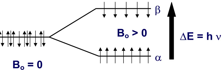
Figure 2. Without an external magnetic field B0 (B0 = 0), there are no energy differences between all the nuclear spins in a bulk sample. After applying an external magnetic field B0 (B0 > 0), the thermal effect generates the population difference between the spin up α and spin down β levels according to the Boltzmann distribution... 11

Figure 3. Laboratory frame and rotating frame in the nuclear magnetic field... 14

At rotating frame, the time dependence of the B1 field will be removed and it will appear to be static... 14

Figure 4. The rotating frame rotates about the z-axis at the frequency of the rf pulse, ωrf. ... 15

Figure 5. On –resonance 90° (a) and 180° (b) rf pulses that flip the nuclear magnetic spins to y΄ and –z axis, respectively... 16

Figure 6. The magic angle spinning scheme in solid –state NMR experiment. (following reference 5) ... 19

Figure 7. The effects of magic angle spinning on homonuclear dipole-dipole interaction. The broad line is narrowed by magic angle spinning rates of the order of the dipolar linewidth or higher. For slow MAS speed, broad spinning sidebands appear, and at very slow speed, there is no big effect of removing any of the effects... 21

Figure 8. High power proton dipolar decoupling removes the effects of proton dipolar coupling from the 13C solid-state NMR spectrum. High power irradiation is applied to the 1_{H spins at the proton on-resonance frequency during the acquisition of the} 13_{C spin} NMR spectrum... 22

Figure 9.Multiple pulse sequences used for removing homonuclear dipolar coupling from solid-state NMR spectrum. In (a) WAHUHA ( after Waugh, Huber, and HAberlen)39 sequence and in (b) MREV-8 (after Mansfield, Rhim, Elleman, and Vaughan)40,41 sequences, all pulses are 90° pulses with the indicated phases, multiple times (as indicated by the arrows.) The MREV-8 sequence is actually a two phase-cycled WAHUHA sequence... 23

Figure 10. Cross polarization achieved by the Hartmann-Hahn condition, γ13CB1 = γ1HB1’ ... 25

Figure 11. Cross Polarization Pulse Sequence... 26

Figure 12. CP/MAS spectrum for hexamethyl benzene (HMB)... 28

Figure 13. Classical flip-flop of two magnetic dipoles... 31

Figure 14. Schematic Representation of 1H spin diffusion process. (following reference 26) ... 33

Figure 16. 2D Solid-State Heteronuclear Correlation pulse sequence (HetCor). Typical experimental parameters include 90° pulse widths 3.2 µs on each channel, spinning speeds 3.5-4.5 kHz, 256-512 scans for each 64 points in t1 dimension, typical

experimental time 12-24 hours. ... 37 Figure 17. PC (poly (bisphenol A carbonate)) and PPO (poly

(2,6-dimethyl-1,4-phenylene oxide)) simulated chain units... 40 Figure 18. Simulated structure for a PPO chain demonstrating how the characteristic monomer dimension x = (lcdc) 1/2 was calculated. ... 41

Figure 19. 2D HetCor spectra obtained for PC with spin-diffusion times of (A) 0, (B) 0.1, (C) 3 ms. Note in particular the time-dependent cross-peak intensities for the CH3

and aromatic CH groups. ... 44 Figure 20. (a) The 13C slices at the methyl 1H peak (top) and the aromatic 1H peak

(bottom) for τm = 0. (b) The 1H slices at the 31 ppm methyl 13C peak (top) and the 128

ppm aromatic 13C peak (bottom) for τm = 0. (c) The 13C slices at the methyl 1H peak (top)

and the aromatic 1H peak (bottom) for τm = 1 ms. (d) The 1H slices at the 31 ppm methyl 13_{C peak (top) and the 128 ppm aromatic} 13_{C peak (bottom) for τ}

m = 1 ms... 45

Figure 21. Spin-diffusion curves for PC constructed from deconvolution of the 1H slices at the methyl (31 ppm) and aromatic (128 ppm) 13_{C shifts in terms of the integrated}

intensity ratio of (Iaromatic / (Iaromatic + Ialiphatic))... 47

Figure 22. 2D HetCor spectra obtained for PPO with spin-diffusion times of (A) 0 ms, (B) 0.05 ms, (C) 3 ms... 50 Figure 23. Complete spin-diffusion curves for the 2D HetCor experiments for PPO. Here the growth of the aliphatic 1H correlation at the 120 ppm aromatic 13C chemical shift is plotted as a function of the square root of the spin-diffusion mixing time... 51 Figure 24. Simulated structure for the PC, where the cylinder inscribes the “effective” monomer size... 53 Figure 25. (top) 2D HetCor spectrum for a monodisperse PS-b-PMMA diblock

copolymer obtained using a 5 ms spin-diffusion time, with the summed cross-peak projection for the 13C dimension shown on the top of the plot. (bottom) Selected 1H slices through the 128 ppm PS peak as a function of spin-diffusion time τ(tau); the dashed line on the contour plot indicates the slice position... 56 Figure 26. Complete spin-diffusion curves for the PS-b-PMMA in which the ratio of ( Ialiphatic / ( Iaromatic + Ialiphatic )) is plotted vs the square root of the mixing time for the 128

indicating how the spin-diffusion curves in subsequent figures were extracted from the 2D experiments. For the MP-WIM HetCor, MAS spinning speeds of 3.5 – 4.5 kHz were used, while the FSLG HetCor data were collected at 12-13 kHz. Quadrature detection in the second dimension (using TPPI) was insured by appropriate phase cycling and data addition for both the MP-WIM and FSLG experiments43,103. Approximately 40 mg of sample in a 4-mm MAS rotor was used for the MP-WIM experiments, whereas only 10 mg was used for the FSLG data (due to confinement in the most homogeneous region of the r.f. coil)... 66 Figure 29. Total spin-diffusion curves obtained using Lee-Goldburg (FSLG) vs.

multiple-pulse Hetcor (MP-WIM) for (a) PS-b-PMMA with a total molecular weight of 50K (25K blocks for each component); (b) PS-b-PMMA with a total molecular weight of 100K; (c) PS-b-PMMA with a total molecular weight of 200K. In (d), a schematic of a typical spin-diffusion curve resulting from the measurement of only interdomain

polarization transfer is shown. The lines are drawn merely to guide the eye in examining the different responses. ... 72 Figure 30. (a) MP-WIM spin-diffusion curves for PS-b-PMMA with a total molecular weight of 50K, in which the same 2D Hetcor data set was analyzed twice (phasing, slice selection, deconvolution, and intensity ratio determination). (b) MP-WIM spin-diffusion curve for PS-b-PMMA 100K with representative error bars determined by triplicate experiments on four randomly selected spin-diffusion mixing times (details described in the text). (c) MP-WIM spin-diffusion curve for PS-b-PMMA 100K obtained at two different MAS speeds. (d) Plot of 128-ppm PS aromatic C-H slice intensity versus MAS speed for MP-WIM spin-diffusion experiment at two different spin-diffusion times... 77 Figure 31. Two dimensional Frequency-switched Lee-Goldburg heteronuclear correlation experiment with Lee-Goldburg cross-polarization pulse sequence. 1H radiofrequency field strength during FSLG evolution period and TPPM decoupling period were set at 90-95 kHz, correspond with π/2 pulse of 2.65-2.75 µs. At 1H LGCP period, radiofrequency field strength is 64-68 kHz, correspond with π/2 pulse of 3.7-3.9 µs.13C ramp CP is used, CP time = 100 us. MAS speed = 13 kHz. Quadrature detection in t1 is achieved by TPPI.

... 84 Figure 32 (a)1_{H Bloch decay spectrum of pure bulk PCL; (b)}1_{H Bloch decay spectrum}

of pure bulk PLLA; (c) 1H Bloch decay spectrum of coalesced PCL/PLLA blend; (d)13C CP/MAS spectrum for the solution PCL/PLLA blend; (e)13C CP/MAS spectrum for the same sample as in (c). Assignments follow the structure schematic (top). Spectra (a) – (c) were acquired with 13 kHz MAS. Asterisks denote spinning sidebands. ... 89

Table 1. 1H rotating-frame spin-lattice relaxation time constants T1ρH (in milliseconds)

for PCL/PLLA blends versus sample preparation method. ... 90 Figure 33. Representative two-dimensional 1H-13C solid-state Hetcor plots of the

aliphatic 13C region for: (a) FSLG/LGCP acquisition on the solvent-cast blend with no spin-diffusion time; (b) same as (a), after 1 ms spin-diffusion time; (c) MP/WIM

acquisition on the coalesced blend with no spin-diffusion time; (d) same as (c), after 1 ms mixing time. 1_{H slices were extracted at 19 ppm and 65 ppm for the spin-diffusion}

analysis. Summed projections from each dimension are shown along the 13C (horizontal) and 1H (vertical) axes... 93 Figure 34. 1HSpin-diffusion curves extracted from slices at the PLLA CH3 signal (19

arrows indicate the predicted equilibrium intensity ratios for intramonomer vs. intermolecular (interdomain) spin-diffusion based on the monomer structures. The dashedline in the short time regime is the regression through the first five points of the curve to the intramolecular equilibrium intensity ratio (0.25). From this latter analysis, the equilibration time for intramolecular spin-diffusion was 20 µs1/2 (τintra vertical arrow).

Additional vertical arrows indicate the equilibration times for intermolecular or

interdomain spin-diffusion between PLLA and PCL in the coalesced (τcoal = 88 µs1/2) and

solution-cast (τsol = 132 µs1/2) blends, obtained by regression of the four experimental

points between the intramolecular and intermolecular plateaus. ... 94 Figure 35. 1HSpin-diffusion curve from pure PLLA () vs. PLLA in the coalesced blend with PCL( ), demonstrating a decrease in the spin-diffusion coefficient D upon blending. The last data point for the PLLA/PCL coalesced blend is already at the

intermolecular equilibrium value, as previously seen in Figure 32. ... 98 The value of DPLLApure = 2.1 × 10-12 cm2 s-1 is in agreement with our previous

determinations of D’s based on intramonomer spin-diffusion94,128. For the higher-Tg

polycarbonate (Tg = 140 ° C) and lower- Tg polyisobutylene (Tg = -70 ° C), the

previously reported spin-diffusion coefficients were 5.1 × 10-12 cm2 s-1 and 4.4 × 10-14 cm2 s-1,respectively. Since the PLLA Tg is intermediate between these two extreme (Tg = 60

° C), an intermediate value of D expected. ... 98 Figure 36. Biexponential fit for 1H spin-diffusion curves extracted from slices at the PLLA CH3 signal (19 ppm) for the coalesced ( ) PCL/PLLA blends at figure 32. The

biexponential equation is f = a*(1-exp (-b*x)) +c*(1-exp (-d*x)), the parameters are as following: a = 2.4302, b = 0.0547, c = -2.2202, d = 0.0495 R2 = 0.948. The solid line is the two-component fit, with the short time response attributed to intramolecular

polarization equilibration, and the long time component to interdomain spin-diffusion. 99 Figure 37. Expanded Hetcor plot of the OCH and OCH2 region of the spectrum showing

that the broad downfield (in the 13_{C dimension) shoulder off the PLLA peak is clearly}

LIST OF TABLES

Table 1. 1H rotating-frame spin-lattice relaxation time constants TρH (in milliseconds)

for PCL/PLLA blends versus sample preparation method. ... 90

Table 2. 1H spin-lattice relaxation time constants T1 (in seconds) for PCL/PLLA blends

Chapter 1. Motivation and Introduction

1. Motivation

The physical properties of solid polymers, such as thermal, mechanical, electrical, optical, barrier, and ageing mostly depend on two aspects. First, they are determined by their molecular structures, which are their internal properties, and can be cautiously controlled by various chemical syntheses. Secondly, their physical properties also strongly dependent on the structural organization of the macromolecules in the solid state, including morphology, local structure, phase behavior, and molecular dynamics1,2,3. To improve and optimize macromolecular behavior and mechanical properties one needs to understand the structure-property relationships. To deepen the knowledge, the focus needs to be on the development of modern experimental techniques, which can probe microscopic and molecular parameters in the solid state1,4 for amorphous macromolecules.

In order to understand the polymers’ physical properties, one can divide them into three categories based on length scales6_{. They are (1) the molecular (microscopic) level,}

level, the crystalline and amorphous regions organize respectively into morphological region.

The macroscopic physical properties of polymers are governed by all three length scale levels. Various experimental techniques can be used to probe the microscopic properties6,7. Fourier transform infrared (FT-IR) 8 and raman spectroscopy9 can determine the molecular scale characterization. Small angle X-ray scattering (SAXS) 10,11, wide angle X-ray scattering (WAXS)12,13,14, neutron diffraction15,16,17,18, electron scattering19 and electron microscopy (TEM19,20, SEM20,21, AFM22) techniques can be used to characterize the macromolecular local order.

X-ray scattering is one of the classic techniques used for polymer characterization. It provides information to answer the question about whether a polymer is crystalline or amorphous, oriented or unoriented and to determine the size of characteristic repeat distances. Also, it can determine the structural information such as the unit cell, space group and atomic coordinates of a crystalline or semicrystalline polymer, which relates to polymer’s atomic scale but is averaged over the sample volume (typically on a scale of

thermodynamics between the protonated and deuterated polymer may be different. This concerns whether the local structures of the polymer have been changed by the insertion of the labeled polymer. Electron scattering and electron microscopy techniques are based on high energy electrons scattering in the polymer structure and the diffraction patterns resemble those obtained from X-rays. Electron scattering is mainly applied to very highly crystalline materials. The resolution of these techniques can be at the 0.1 nm level and provides useful information that is below the resolution limit of the conventional optical microscope. Transmission electron microscopy (TEM) has been used to visualize the chain packing in polyethylene type polymer20. This method required the section of the samples below 100 nm, which allow the electron beam to pass through the material. The TEM method can provide electron diffraction data that can be used to calculate the molecular spacing in crystalline phases in the polymer material. The alternative approach to electron microscopy is scanning electron microscopy (SEM) 20. In SEM the backscattered electrons contain an energy which is the characteristic of the atoms that produce the scattering21. Since the resolution of light atoms such as carbon and oxygen at SEM is very poor, this method is only useful for heavy atoms.

In the past 20 years, solid state nuclear magnetic resonance (SSNMR) advancements have added new possibilities in polymer physical and chemical property characterizations1-4,23,24.

microscopy, and dielectric or mechanical relaxation. However, an experimental determination and characterization of local structure, and the resulting morphology at length scales shorter than about 50 nm in amorphous polymers and other noncrystalline compounds is difficult. In addition, the information content in small-angle X-ray diffraction is often insufficient due to a low contrast4.

Recently, solid-state spin diffusion NMR methods have been introduced to interrogate the essential characteristics of the local structure, as well as the morphology of the amorphous macromolecules and their blends. These spin diffusion methods determine the time dependent spin diffusion polarization transfer under the influence of nuclei dipolar interactions. From this, the distance information (domain size for blends, composites, and copolymer) can be obtained with the introduction of a spin diffusion coefficient. Some excellent reviews have been published in this area25,26.

2. History of NMR

2.1. Unique features of NMR

NMR was rapidly accepted in physics and chemistry and has been applied in many directions because of its inherent, unique features. Since the radiation (Megahertz frequencies) used in NMR experiments is monochromatic, it avoids the burden to render broad-band radiation in other spectroscopic experimental techniques. There are only very small energy changes involved in the transition between nuclear spin energy levels. Thus, the NMR experiment causes only a slight perturbation of the system in contrast to optical spectroscopy experiments. As a result, the information obtained from NMR experiments will represent the bulk properties of the macromolecules. A related point in the NMR experiment is that the spacing of the nuclear spin energy levels increases with the applied external magnetic field, B0. Also, the Boltzmann factor is larger at higher fields,

increasing the sensitivity further.

2.2. Discovery of NMR

Discovery of Nuclear Magnetic Resonance

Fourier Transform NMR Spectroscopy (FT-NMR)

Nuclear Magnetic Resonance (NMR) spectroscopy is one of the most powerful tools in modern science. Since its discovery, NMR has found applications from physics to chemistry, biosciences, material research and medical diagnosis.

The development of NMR as a routine analytical technique in these fields parallels the development of electromagnetic technology. During World War II, Purcell worked on the development and application of RADAR at MIT's Radiation Lab. His work during that project was mainly concerned with the production and detection of radiofrequency energy and the absorption of such energy by matter. This project preceded the discovery of NMR and contributed to his understanding of NMR and related phenomena.

Throughout the next several decades, NMR spectroscopists mostly utilized a technique known as continuous wave (CW) spectroscopy. In cotinuous wave spectroscopy, either the magnetic field was held constant and the oscillating field was swept in frequency to plot the on-resonance portions of the spectrum, or more frequently, the oscillating field was kept at a fixed frequency, and the magnetic field was swept through the transitions. The limitation of this technique is that it probes each of the frequencies in succession, resulting in a poor signal-to-noise (S/N) ratio.

the development of modern computers capable of performing the computationally-intensive mathematical transformation of the data from the time domain to the frequency domain, to produce a spectrum.

In the fall of 1963 Richard R. Ernst at Varian Associates in Palo Alto under the guidance of Dr. Weston Anderson, found FT-NMR can significantly increase NMR’s signal-to-noise ratio by irradiating the sample with a short radiofrequency pulse. Detectors record the decay of this excitation as a time-dependent pattern, known as the free induction decay (FID). This time-dependent pattern, when processed through the Fourier transform, reveals the frequency-dependent pattern of nuclear resonances, the NMR spectrum. According to Fourier theory, the shorter the pulse, the broader the range of frequencies it contains. R. R. Ernst was awarded the Nobel Prize for chemistry in 1991 "for his contributions to the development of the methodology of high resolution nuclear magnetic resonance (NMR) spectroscopy"27.

The use of pulses of various shapes, frequencies, and durations, in specifically-designed patterns, gives the spectroscopists great flexibility in determining what portions of a molecule, or what intra- and intermolecular dynamic processes, to study. The gain in sensitivity over several decades has opened many new research directions in the following several decades till now, such as the application of high resolution NMR spectroscopy to molecules adsorbed on solid surfaces, and biological macromolecular NMR.

Two and Multi-dimensional NMR Spectroscopy

(t2), and the second dimension is based on the time differential between the pair of pulses

(t1). The final spectra will be Fourier transformed, expressing the first and second

dimension as frequencies (F1 and F2). In multidimensional nuclear magnetic resonance

spectroscopy, there will be a sequence of pulses, and at least one variable time period. For example, in 3D, two time periods will be varied, while in 4D, three will be varied.

These time intervals allow spin magnetization transfer between nuclei in the external magnetic field and therefore NMR spectroscopists can detect the interactions between nuclei that generate the spin magnetization transfer. The kinds of interactions that can be detected are usually divided into two categories. The first is through-bond interactions, such as J coupling interaction. And the second is through-space interactions, such as dipole-dipole interaction, an example of which is nuclear Overhauser interaction.

Development of Powerful Magnets

3. Short review of the solid-state NMR theory

3.1. Basics of NMR

Classical vector model of the nuclear spin5, 30, 31

When looking at a classical model of NMR, we will only consider the net nuclear spin magnetization coming from the nuclei in the sample and its behavior in magnetic fields. Without an applied external magnetic field, all nuclear spins are degenerated meaning they are disordered in their ground states with no energy differences between them (Figure 1A). In this dissertation, we will exclusively deal with spin ½, therefore, here we will only consider the spin ½ conditions. All the nuclear spins have nuclear magnetic moment µ, when they are placed in a strong external magnetic field B0, they

will reorient either parallel or anti-parallel to the applied nuclear magnetic field B0 from

disordered ground states. Figure 1B shows the nuclear spin reorientation after they are placed in an external magnetic field B0.

A. B.

Figure 1. The classical vector model of nuclear spins in a sample.

A. In the absence of an applied magnetic field, the nuclear spins (represented by vector arrows) are disordered in their ground states, there are no energy differences between them, and as a result, there is no net nuclear magnetization in the system.

B. After applied an external magnetic field B0, the nuclear spin vectors reorient

parallel or anti-parallel to the applied B0 field according to the Boltzmann distribution

thermal effects, creating net nuclear magnetization.

The relationship between the nuclear spin magnetic moment µ and angular momentum L can be defined by the following equation:

µ = γ L (1)

In this equation, γ is the nuclear spin’s magnetogyric ratio. The magnetogyric ratio γ

is individual to each type of nuclei. In NMR, the applied magnetic field is generally placed along the z direction. Following the application of a strong external magnetic field B0, the nuclear spins will precess about this field at the frequency which is defined by the

equation:

ω = - γ B0 (2)

The frequency ω is called the Larmor precession frequency of the nuclear spins, γ is the magnetogyric ratio of the nuclei, and B0 is the applied magnetic field strength. If ω

has the traditional units of rad sec-1 and the magnetic field B0 has units of Tesla (1T = 104

Gauss), the magnetogyric ratio γ will have the units of rad sec-1 T-1. Thus, the proton

frequency ω in the applied magnetic field B0 will be ω = 2.6751 * 108 B0 rad sec-1. Since

NMR spectroscopists like to use f0 (units is Hz) instead of ω (rad sec-1) for the Larmor

B

= 0

B

> 0

∆

E = h

ν

α

β

Here, the proton Larmor frequency f0 will be f0 = 42.575 B0 MHz, where units of B0

is still Tesla. For example, when B0 = 7.03 Telsa, the proton Larmor frequency f0 will be

300.00 MHz. The direction of the bulk spin magnetization is anti-parallel to B0 when γ is

negative, such as electron. While it will be parallel to B0 when γ is positive, such as 1H,

and 13C.

Boltzmann distribution and the Spin temperature29

After applying an external magnetic field B0, an energy difference between the two

states of the nucleus (spin up α and spin down β) is created. It is noticed that there are more nuclei in the lower level (spin up α) than the upper level (spin down β), though the population differences are so small that there is generally only one more nuclei in the lower level in one million nucleus bulk samples.

Figure 2. Without an external magnetic field B0 (B0 = 0), there are no energy

differences between all the nuclear spins in a bulk sample. After applying an external magnetic field B0 (B0 > 0), the thermal effect generates the population difference

between the spin up α and spin down β levels according to the Boltzmann distribution.

Nβ/ Nα = e -∆E / kT = e hγ / kT (4)

Under general conditions the value of hγ will be much smaller than the value of kT, so the Boltzmann distribution equation can be simplified to the following:

Nβ/ Nα = 1 - hγ / kT (5)

When applying the Boltzmann distribution to the nuclear magnetization system, it will be very useful to define a spin temperature term “Ts”, which can simulate the general temperature term in the regular thermal equilibrium system.

Nβ/ Nα = e -∆E / kTs = e hγ / kTs (6)

We can see that it is very convenient to use the spin temperature Ts to describe the phenomenon of an NMR experiment. When the experiment starts, the radio frequency irradiation will find a population difference between the upper and lower levels. There are more spins in the lower energy state (spin up α) than higher energy state (spin down

β). The effect of the rf irradiation is that it makes more of the spin up (α) go up than the spin down (β) to go down. After several transitions take place, Nαwill decreaseand Nβ

system and produce no more net absorption. At that time, the spin system has reached saturation.

The effect of radiofrequency pulses

An electromagnetic wave, such as a radiofrequency (rf) pulse can excite nuclear magnetization. When the nuclei are excited, they will absorb energy and jump from lower levels to higher levels, and eventually they will relax back to lower levels and emit extra energies. The NMR detects the absorption of the electromagnetic radiation, and converts it to signal seen in an NMR spectrum. Only nuclei with spin number (I) ≠ 0 can absorb/emit electromagnetic radiation. This radiofrequency wave generates an oscillating magnetic field B1, which interacts with the nuclei in addition to the static applied external

nuclear magnetic field B0 in the NMR experiment. The rf pulse is arranged in a position

so that its nuclear magnetic field can oscillate along a direction perpendicular to z and B0

field. The B1 oscillating field can be divided into two frequency components which rotate

about B0 field in opposite directions. We defined the two frequencies as ±ωrf. When

introduced a rotating frame of reference which rotates at frequency ωrf aroundthe B0

laboratory frame, the effect of this B1 field will be most easily seen. In this rotating frame

z

x

M

y

B

ω

Laboratory Frame

z

x

M

y

Rotating Frame

Figure 3. Laboratory frame and rotating frame in the nuclear magnetic field.

At rotating frame, the time dependence of the B1 field will be removed and it will appear to be static.

On resonance, off resonance rf pulse and flip angle

Let’s look at the effect of a rotating frame in the condition without the rf pulse. When the nuclear spin vector is put in the B0 field, a static, uniform nuclear magnetic

field, the nuclear spin vector M will precess around B0 at a frequency ω0 in the laboratory

frame. Now, if an on-resonance pulse is applied, meaning ω0 = ωrf, the nuclear spins will

appear stationary in the rotating frame. The only effective field left in the rotating frame will be the B1 field, while the B0 field is removed in this frame. The nuclear spins will

precess about the B1 field at the following frequency:

ω1 = γB1 (7)

Here, ω1 is known as the nutation frequency. The pulse does not have to be applied

be many cases in the solid-state NMR experiments when pulses are applied off-resonance. For example, in the later chapters, the frequency switched Lee-Goldburg cross polarization experiment has to apply the LG frequency pulse, which is an off-resonance pulse. In the rotation frame, the Larmor precession frequency is reduced from ω0 to ω0 – ωrf about B0, which means the effective field along the z axis in the rotation frame is (ω0

– ωrf) / γ, rather than zero. As a result, the total nuclear magnetic field in the rotating

frame can be expressed with the following equation:

2 ₁2

0 2

0 (1 / ) B B

B_eff = −ω_rf ω + (8)

The magnetization will precess around the resultant effective field Beff as shown in

Figure 4.

Figure 4. The rotating frame rotates about the z-axis at the frequency of the rf pulse,

ωrf.

The magnetic field B1 due to the applied rf pulse appears static in the rotating frame.

While the external static field B0 is reduced to B0(1-ωrf /ω0) in the rotating frame. The Beff

is the net effective field that the nuclear spin magnetization precesses around.

z

x

The flip angle, θrf, is the angle that the on-resonance pulse turns the nuclear

magnetization during time τrf:

θrf = ω1τrf = γB1τrf (9)

Thus, a 90° pulse, or π/ 2 pulse is the rf pulse that flips the nuclear magnetic spin θrf = π/ 2 or 90° from B1 field. If B1 field points in x’ direction, the magnetization will flip

from the z-axis to y΄ axis. A 180° or π pulse will flip the spins to the –z axis.

Figure 5. On –resonance 90° (a) and 180° (b) rf pulses that flip the nuclear magnetic spins to y΄ and –z axis, respectively.

Introduction

A solid-state NMR spectrum is much harder to acquire as opposed to a solution-state NMR spectrum. Mainly, in solution NMR, rapid polymer chain motion averages the chemical shift anisotropy and the dipolar interactions to almost zero. In solids, the polymer matrix restricts chain motion, and high-resolution spectra can be observed only after using rapid magic angle spinning to average the chemical shift anisotropy and high-power irradiation during signal acquisition to average the 1H-13C dipolar interactions. In some cases more sophisticated NMR methods are used, usually consisting of applying a series of pulses in which the phases are alternated to remove a particular type of interaction. For example, in experiments where spin diffusion would complicate the results, such as the multiple pulse HetCor pulse sequence, it is possible to apply a series of pulses to the protons that quench spin diffusion. In other experiments, such as the 2D exchange pulse sequence, it is possible to obtain information about oriented polymers by synchronizing the pulses and signal acquisition to the sample rotation. In frequency and phase switched Lee-Goldburg HetCor experiments one uses the combination of complex off-resonance rf pulses and fast magic angle spinning to suppress the homonuclear and heteronuclear dipolar interactions.

crystalline polymers as opposed to amorphous materials because they exist in a more uniform environment. The polymer matrix restricts chain motion so the γ-gauche effects are not averaged as in solution, thus the lines of amorphous polymers are inhomogeneously broadened by γ-gauche effects from a distribution of conformations.

In solid-state NMR, generally we will have to deal with anisotropic powder samples. The resultant solid-state NMR spectrum of a powder sample contains broader lines, in other words “powder patterns’. During the last 20 years, solid-state NMR spectroscopy gained a manifold achievement in both signal intensities and spectral resolution. The improvements were achieved via various pathways, such as macroscopic sample rotation (Magic-Angle-Spinning and Off-Magic-Angle-Spinning) 33,34, combining high-speed mechanical rotation of the sample with ingenious manipulations of the nuclear spins such as multiple-pulse irradiation, high-power decoupling and cross polarization35, two-dimensional and higher-two-dimensional NMR techniques. 36,37,38,26

Magic angle spinning

Removal of chemical shift anisotropy and heteronuclear dipole-dipole interaction

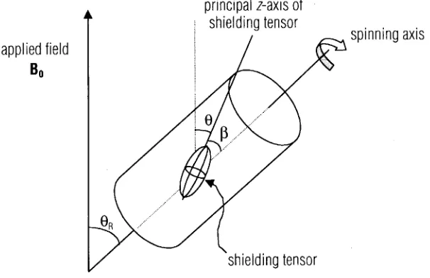
Figure 6. The magic angle spinning scheme in solid –state NMR experiment. (following reference 5)

The sample spins in a cylindrical rotor about a spinning axis oriented at the magic angle (θR = 54.7°) with respect to the applied magnetic field B0.

In solution NMR spectra, due to the rapid tumbling of the molecules, the effects of chemical shift anisotropy (CSA) and dipolar interaction almost disappear. The rate of change of molecular orientation is fast relative to the effect of CSA, and dipole-dipole interaction, thus averaging the (3cos2θ – 1) dependence of the transition frequencies. Here, the angle θ is the angle of the shielding tensor with respect to the applied field B0.

at the magic angle (θR = 54.7°) to the applied magnetic field B0, the average of (3cos2θ –

1) in these conditions can be shown with the following equation:

(3cos2_{θ −}1)₌ (3cos2_{θ −}1)(3cos2_{β −}1)

R (10)

Angle β and θR are definedin Figure 6. Since θR is set tobe the magic angle 54.7°, then

(3cos2_θ

R – 1) = 0, thus the average of (3cos2θ – 1) is zero too. In conclusion, providing

the MAS spinning speed is fast enough, the effect of CSA and dipole-dipole interaction will approach to zero.

Fast MAS for removal of homonuclear dipole-dipole interaction

Figure 7. The effects of magic angle spinning on homonuclear dipole-dipole interaction. The broad line is narrowed by magic angle spinning rates of the order of the dipolar linewidth or higher. For slow MAS speed, broad spinning sidebands appear, and at very slow speed, there is no big effect of removing any of the effects.

High power proton dipolar decoupling

1

_H

13

_C

In the case of dipolar-coupled 1H and 13C spin pairs, where 13C spins’ signals are needed to be observed, the application of high power decoupling will consist of applying a continuous irradiation of very high power (100-1000 watts) at the frequency of the proton resonance. In other words, following the 13C pulse sequence, while the 13C FID is being acquired, continuous high power 1H irradiation decoupling is applied.

Figure 8. High power proton dipolar decoupling removes the effects of proton dipolar coupling from the 13C solid-state NMR spectrum. High power irradiation is applied to the 1H spins at the proton on-resonance frequency during the acquisition of the 13C spin NMR spectrum.

Multiple pulse decoupling sequences

Figure 9.Multiple pulse sequences used for removing homonuclear dipolar coupling from solid-state NMR spectrum. In (a) WAHUHA (after Waugh, Huber, and HAberlen)39 sequence and in (b) MREV-8 (after Mansfield, Rhim, Elleman, and Vaughan)40,41 sequences, all pulses are 90° pulses with the indicated phases, multiple times (as indicated by the arrows.) The MREV-8 sequence is actually a two phase-cycled WAHUHA sequence.

Many useful multiple pulse sequences exist in literature. The first, and also one of the simplest, is the WAHUHA sequence, shown in Figure 9 (a). The MREV-8 sequence is a modification of the simple WAHUHA sequence, is also widely applied. In a later section, we will use the BLEW-1242, 43 sequence to remove homonuclear dipolar coupling during the two dimensional heteronuclear correlation pulse sequence. The multiple pulse sequences are arranged in such a way that the effect of the dipolar Hamiltonian on the nuclear magnetization approaches zero.

Cross polarization and Hartmann-Hahn condition

In numerous NMR experiments, there is a need to transfer energy between different sets of magnetic nuclei with different precession frequencies in order to enhance the signal. This can be achieved via cross polarization under the Hartmann-Hahn condition44. Transfer of energy from one kind of nuclei to another is facilitated if the two different nuclei have the same resonance frequency. The most common example of the cross polarization energy transfer is between 1H and 13C. Clearly, since the proton resonance frequency is a factor of four larger than that of 13C, the transfer of energy between them is forbidden. We can think of an experiment which places 13C nuclei in a high magnetic field and the 1H nuclei in one-fourth as strong a field so as to achieve the same frequency. The condition here is the following:

γ13CB0 = γ1HB0’ (11)

Obviously, it is difficult to have two magnetic fields differing by a factor of four at the protons and 13C nuclei in the same molecules, but these difficulties are overcome under the Hartmann-Hahn condition. The first step in the Hartmann-Hahn process is to bring each set of nuclei to XY plane by a π/2x degree pulse. Next, each set of nuclei needs

to be spin-locked to the Y axis by either a series of πy pulses or equivalent continuous

irradiation at the appropriate frequencies, then achieving the following state:

13

_C

X

Y

Z

1

_H

ω

(

H) =

ω

(

C)

Figure 10. Cross polarization achieved by the Hartmann-Hahn condition, γ13CB1 = γ1HB1’

The Hartmann-Hahn condition is demonstrated in Figure 10. During these conditions, both sets of nuclei, within their respective rotating frames, precess with the same frequency about the Y-axis, thereby providing an opportunity for exchange of energy via coupled spin flip-flops.

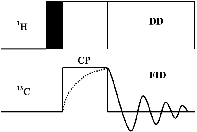
CP pulse sequence

Figure 11. Cross Polarization Pulse Sequence.

After a π/2 excitation pulse on protons, transverse 1_{H magnetization is locked while} 13_{C magnetization is created if the spin lock fields match the Hartmann-Hahn condition.}

Subsequently, the signal is observed under high power dipolar decoupling. The CP experiment is performed under magic angle spinning to attain the best signal. In combination with magic angle spinning, high resolution conditions are obtained for solid samples22, yielding isotropic signals with the characteristic chemical shift dispersion of

13_{C and a typical linewidth of ~1 ppm. The CP/MAS experiment is the basis for many}

two- and multi-dimensional solid-state NMR experiments.

Experimental parameters

The MAS rotation frequency should be chosen high enough to average out the chemical shift anisotropy but not too high because sample heating due to rotor friction occurs. Typically, values between 3 and 6 kHz are reasonable for solid samples at high

CP

Π

/2

FID

1

_H

13

_C

magnetic field. The typical pulse length for the 1H 90° excitation pulse should be on the order of 3-4 µs. The spin lock field on one channel should be set to approximately 50 kHz, while the corresponding spin lock field of the other channel is best determined experimentally for each sample. (the Hartmann-Hahn condition turns out to be dependent on the MAS frequency and shaped spin lock pulses may become necessary for efficient polarization transfer.) 23 Modern spectrometers allow for parameter optimization by sweeping through the power setting for the spin lock until maximum signal intensity is found. In organic solids, typical contact times to achieve maximal intensity are in the range of 0.5 to 1 ms. During acquisition, high power 1H decoupling with a typical radio frequency (rf) field strength of 60-80 kHz should be applied. Best results are obtained with TPPM (two pulse phase modulation) scheme24. Typical signal acquisition times are determined by the linewidth but should not exceed ~25 ms to avoid rf heating. A relaxation delay of 2-5 s between successive scans should be allowed for protons to fully relax and to prevent sample heating.

Figure 12. CP/MAS spectrum for hexamethyl benzene (HMB)

3.3. Special solid-state NMR sequences

3.3.1. T1, T2 and T1ρ

T1 relaxation (also called longitudinal relaxation, spin lattice relaxation time45) is a

measure of the relaxation rate along the z axis. During this relaxation, the nuclear magnetization will lose its energy in the system to the surroundings (lattice) as heat. Examples of energy loss mechanisms include nuclear spins dipolar couple with other spins, or interaction with paramagnetic particles, etc. There are two ways to measure the T1 relaxation time. The first is the inversion-recovery pulse sequence, which consists of

180° - τ - 90° (observe) 46-48. The180°x’ flip pulse inverts the M0 (Magnetization) to the –

z axis, and then it decays exponentially back to M0 as described by the following

equation:

Mt = M0 {1 – 2 exp [- (t /T1)]} (13)

From the equation, we can see that when M is fully inverted, M will relax from - M0

through zero to +M0. And when we get the time (tz) required for M to reach zero, we can

calculate T1 by the equation:

At this point, there is no X/Y magnetization, so there will be no way to see the signal in order to quantify T1. To solve this problem, we can apply a 90° pulse at particular

intervals after the original 180° pulse. This way, the relaxed magnetization is flipped to the transverse plane (XY plane), and the receiver coil can detect the signals. A second way to measure the T1 relaxation time is via the saturation-recovery pulse sequence. A

limitation of using this method to measure T1 is that spin- spin relaxation (T2) in the xy

plane must be much faster than the spin- lattice relaxation (T1) in the z direction. The

pulse sequence is 90° - τ - 90° (observe). In this case, if the magnetization is placed in the xy plane by applying a 90° pulse, it will decay to zero before significant spin- lattice relaxation (T1) occurs and then the magnetization will grow back to equilibrium in the z

direction. Finally a 90° pulse is applied to acquire the signal. In order to make sure that the system is fully saturated, there is a preparation step which can be achieved using two common methods. Usually, one can apply a series of hard pulses with only short delays between them so that there is not enough time for the system to return to equilibrium and the whole spectrum becomes saturated. The hard pulses are always set up using 90° pulses. An alternative way is to use broadband 1_{H decoupling, which will rapidly saturate}

the proton magnetization. The equation to calculate or map the spin –lattice relaxation time (T1) in the saturate-recovery pulse sequence is the following:

Mt = M0 {1 – exp [- (t /T1)]} (15)

T2 relaxation (also called transverse relaxation, spin-spin relaxation45) is used to

measure the rate of relaxation in the xy plane. T2 relaxation does not involve energy

imperfections have a serious effect on T2 measurements. The observed decay is always

faster than 1/T2 because of the magnetic field inhomogeneity. Here each nuclear spin in

the bulk sample experiences a slightly different local B0, thus each spin will precess at a

slightly different frequency from the other nuclear spins. The result is a “fanning out” with a loss in phase coherence. We can use the Carr-Purcell-Meiboom-Gill (CPMG) pulse sequence to eliminate this inhomogeneous magnetic field contribution and get the real value of T2. The CPMG pulse sequence is the following: 90°+x -τ – [180°y- 2τ] n -

180°y - τ (Acq). The pulse sequence generates a spin echo pulse in the transverse plane

(xy plane), and refocuses the magnetic field inhomogeneity effect by repeating – [180°y - 2τ] n times. The value of T2 can then be calculated by this equation

My (t) = My (0) exp [-(t /T2)] (16)

T1ρ is known as the spin lattice relaxation time in the rotating frame49-51. The pulse

sequence is 90ºx-B1y-τ-observe. An on-resonance 90º pulse is first applied along x’ to

bring the magnetization along y’. The phase of this pulse is then shifted by 90º so that it is now applied along y', followed by a 90º shift pulse or a “spin locking” pulse52-60. The magnetization is now spin locked by B1y and it will undergo no precession in the rotating

frame. However, the magnitude of the magnetization is far larger than can be maintained by B1, since it was developed in B0, which is several orders of magnitude greater than B1.

Therefore, with time, the magnetization will decay with time to a value of (B1/B0) M0,

which is very small. This is very important for the T1ρ measurement because in the

absence of this spin locking pulse, there would be simple decay of the y' magnetization due to T2 relaxation processes. The spin-lattice relaxation in the rotating frame is

I

I

I

I

My (t) = My (0) exp [-(t /T1ρ)] (17)

3.3.2. Spin diffusion and spin-diffusion solid-state NMR

The next focus will be on spin-diffusion in solid-state NMR experiments applied to amorphous polymers, blends and composites. This method is used to interrogate the local structure, dynamics, miscibility and the relationship between them. This method is very attractive since it does not require isotopic labeling, 61-63 a neutron source, or any special sample preparation treatments.

Bloembergen first introduced the term “spin diffusion” in 194764. Spin diffusion is actually a result of oscillating local transverse dipolar fields. Figure 13 shows the classical flip-flop of two magnetic dipoles. Many oscillating fields can lead to spin diffusion relaxation, also referred to as spin diffusion equilibrium.

Figure 13. Classical flip-flop of two magnetic dipoles.

phenomenon is actually based on reversible coherent dipolar evolution65 and does not represent a diffusion process in the classical sense. “Dipolar magnetization transfer” is a more correct description. The characteristics of the dipolar magnetization transfer depend somewhat on the spin species concerned, in particular on its abundance and on the strength of the dipolar coupling compared with other interactions. The most important spin diffusion processes in polymeric systems are among 1H and 13C nuclei. Here we will focus on the 1H spin diffusion process. Since the proton-proton dipolar coupling in typical organic polymers is by far the more dominating interaction, this allows for the 1H spin diffusion process to be very efficient. The time dependence of the 1H spin diffusion process contains information on the domain sizes in heterogeneous materials, for example, in structures with small domains, the magnetization equilibrates between domains faster than that in systems with large domains67-71. The spin diffusion equilibrium occurs via the shortest paths, or in other words, spin diffusion can probe a “typical smallest diameter”. For example, 1H spin diffusion can probe domain diameters from about 0.5nm to 200 nm. In the range below 5 nm, the “domain” may often be more correctly denoted as heterogeneities. However, spin diffusion is equally efficient for domains and heterogeneities.

Spin diffusion experiments are exchange experiments, consisting of an evolution or selection period, a mixing time (tm), and a detection period. Figure 14 shows the

Figure 14. Schematic Representation of 1H spin diffusion process. (following reference 26)

In order to let the spin diffusion occur, a spatially inhomogeneous distribution of z magnetization must be generated during the evolution period. In the most favorable case, the magnetization of one component is selected, while the magnetization of the rest of the components in the polymer is suppressed. During the exchange process (tm), the

magnetization of the selected component (denoted as the source region) diffuses out of the source region into its surrounding initially devoid of magnetization. Next, the distribution of all magnetization components in the sample is monitored in the NMR spectrum. For small domains, the magnetization equilibrium will occur fast, while in large structures, the magnetization from the source can only slowly penetrate into relatively thin boundary layers of the other domains. Consequently, the tm dependence of

the spin diffusion exchange is reflected in the spectrum intensities taken after the mixing

Selection Detection Spin diffusion mz mz x mz x mz x mz x x

NMR spectra

_t

(

π

/2)

(

π

/2)

(

π

/2)

τ

In order to experimentally describe the observed diffusive behavior of z magnetization transfer, here, we introduce the spin diffusion coefficient D, which can be determined as

D = Ω * a2 ₍₁₈₎

The term Ω is the spin magnetization diffusion rate, corresponding to the rate of the dipolar coupling, and a is the spacing distance between the spins.

3.3.3. Goldman-Shen experiment – the simplest 1H Spin Diffusion Experiment

The selection of 1H magnetization in spin-diffusion experiments can be based on differences in the decay of the transverse proton magnetization, which is due to the differences in the dipolar coupling. This is the basis of the Goldman-Shen experiment66. Figure 15 shows the principles of the Goldman-Shen experiment, which is the simplest

1_{H spin diffusion experiment, and is applicable to systems consisting of both rigid and}

Chapter 2. New Method for Determination of

Spin-Diffusion Coefficients

1. NMR method: 2D solid-state heteronuclear 1H-13C Correlation experiment

Rigid, high Tg polymers, such as poly (bisphenol A carbonate) (PC) and poly (2,

6-dimethyl-1, 4-phenylene oxide) (PPO), have much longer correlation times of motions, and similar T2 values, due to stronger homonuclear dipolar interactions. Due to these

properties, methods such as the dipolar filter sequence or traditional Goldman-Shen sequence are not applicable for generating a 1H polarization gradient within the monomer units of such rigid, high Tg, amorphous polymers.

behavior is representative exactly of the bulk polymer. Another advantage is that the pulse sequence separates the proton resonance over a much larger 13C chemical shift range, therefore, this technique can provide the well-resolved proton chemical shift information whereas it is impossible with any standard, 1D spectroscopic technique. As such, this technique may detect different polarization transfer processes occurring simultaneously over different length scales in blends or block polymers. The complete experiment is illustrated in Figure 16.

Figure 16. 2D Solid-State Heteronuclear Correlation pulse sequence (HetCor). Typical experimental parameters include 90° pulse widths 3.2 µs on each channel, spinning speeds 3.5-4.5 kHz, 256-512 scans for each 64 points in t1 dimension, typical

experimental time 12-24 hours.

τ

n 63˚

τ

13

_C

BLEW-12 BB-12

WIM-24

1

_H

90˚ 90˚

_t

t

The HetCor pulse sequence has four parts including preparation, evolution, mixing and detection, which are common to virtually all 2D NMR experiments. From Figure 16, it can be seen that at first the spin system is prepared by a single π/2 pulse, followed by the evolution time during which the protons are allowed to evolve in order to “label” them according to their chemical shift. After the evolution period, a spin diffusion time is inserted during which the 1H spin magnetization diffuses to other 1H nuclei in the polymer efficiently according to the distance between them. Then, a special cross polarization period is applied to transfer polarization selectively from the protons to the carbon spins via the heteronuclear dipolar interaction. Finally, the 13C FID is acquired with proton decoupling. During the entire experiment, the sample is rotated at the magic angle in order to suppress broadening due to chemical shift anisotropy86.

Phase cycling is added to the pulse sequence to suppress potential artifacts. In order to obtain a useful HetCor spectrum, it is necessary to effectively suppress both the 1H- 1H homonuclear dipolar interaction and the 1H- 13C heteronuclear dipolar interaction during the evolution period. The HetCor pulse sequence applies the BLEW-1242 _{sequences (a}

windowless multiple-pulse decoupling sequence) to proton spins, while simultaneously applying the BB-12 (a windowless multiple-pulse decoupling sequence by Burum and Bielecki) to 13C spins. The BLEW-12 sequence suppresses homonuclear dipolar coupling, and BB-12 averages out the heteronuclear dipolar coupling, and also suppresses

13_C-13_{C homonuclear dipolar coupling. To maintain the} 1_{H magnetization purely from its}

the mixing period. Also, the cycling of the overall 13C WIM-2484, 85 can eliminate any quadrature interactions, which might otherwise result from an improperly balanced receiver.

All the experiments were done on a Bruker DSX-300 instrument. The π/2 pulse widths were 3.2 µs on each channel. The experimental verification of proper HetCor performance was done using monoethyl fumarate (fumaric acid monoethyl ester). The carbon correlations to both olefinic and acidic protons were observed87. The chemical shift-scaling factor in the 1H dimension was measured experimentally to be 0.42, close to the theoretical 0.47 value. The proton frequency was shifted off-resonance by 5 kHz from the carrier to avoid any zero frequency artifacts and take advantage of second averaging effects. The spinning speed was set to approximately 3.5-4.5 kHz. The spinning speed value is a good compromise between the need to suppress the 13C spinning sidebands and ensuring good polarization transfer performance. The spinning speed periods (285-333

µs) were larger than twice the WIM cycle length (total cross polarization time equals 76.8

µs), therefore preventing signal elimination or attenuation due to a refocusing of the 13C-

1_{H dipolar interaction at the end of each rotor period. 256-512 scans were taken for each}

of 64 points in the t1 dimension, and recycle delays of 3-4 s were used. The total

experiment time was typically 12- 24 hours. Quadrature detection was maintained in the t1 dimension via TPPI (time-proportional phase incrementation). The data were processed

with 50 Hz line broadening and zero filling to 1024 points in the t1 dimension prior to

Fourier transformation.

2. Polymers

The polymers investigated were poly (bisphenol A carbonate)(PC), and poly (2,6-dimethyl-1,4-phenylene oxide)(PPO). The molecular weight of PC and PPO were 100,000 g/mol and 60,000 g/mol, respectively. They are used without any further modification. Figure 17 shows the monomer structures of PC and PPO.

Figure 17. PC (poly (bisphenol A carbonate)) and PPO (poly (2,6-dimethyl-1,4-phenylene oxide)) simulated chain units.

3. Simulation of polymer chain units

Monomer size was determined via molecular chain dynamics calculations and dimensional measurements on chains with degree of polymerization = 100, using Insight II molecular modeling package (Polymer version 3.0.0) with PCFF force field parameters running on a Silicon Graphics IRIS Indigo workstation. Energy minimization was computed with 5000 iterations of an adjusted basis-steepest descents algorithm. Dynamics simulations were carried out at a constant temperature of 300K for 5 ps with time step of 1 fs. The characteristic dimension of the monomer x is defined as follows:

PC _PPO

O C

C CH3

CH3

O

O n

CH3

CH3 O

x = (lc*dc) 1/2 (19)

Here, lc and dc are the length and diameter, respectively, of the cylinder that inscribes

the space-filling dimensions of the monomer. From this model, we extract xPPO=0.59 nm

and xPC= 0.61 nm. Figure 18 shows the simulated structures of PPO.

Figure 18. Simulated structure for a PPO chain demonstrating how the characteristic monomer dimension x = (lcdc) 1/2 was calculated.

4. Data analysis and Discussion

As stated in chapter 2.1, the 2D solid-state HetCor experiment is particularly useful for these rigid, high Tg, amorphous polymers.

Figure 19 shows selected 2D HetCor spectra for neat PC obtained with 0, 0.1, and 3 ms spin diffusion times. The horizontal axis (F2) corresponds to the 13C chemical shift

range (0 to +160 ppm), and the vertical axis (F1) corresponds to the proton chemical shift range (-5 to +15 ppm). Contour spots in the spectra result from individual 13C-1H pairs, correlated by the through-space 13C-1H dipolar interactions. The chemical shift of the 1H and 13C for each pair can be obtained from the F1 and F2 axes, respectively. Horizontal (13C) and vertical (1H) projections of the two-dimensional spectra are shown above and to the left. At τ = 0 (Figure 19A), we can observe that there are no aromatic cross-peaks for the CH3 peak (at 31 ppm) and for the quaternary isopropylidene carbon at 42 ppm, and

A

B

C

ppm

150 100 50 _ppm

15 10 5 0

ppm

150 100 50 _ppm

15 10 5 0

ppm

15 10 5 0 Aromatic

Figure 19. 2D HetCor spectra obtained for PC with spin-diffusion times of (A) 0, (B) 0.1, (C) 3 ms. Note in particular the time-dependent cross-peak intensities for the CH3

and aromatic CH groups.

From these observations, we find that without the spin diffusion time, the protonated sites (bond length ~0.108 nm) are nearly fully polarized and show strong intensities, while the nonprotonated sites with nearest neighbor protons (0.2- 0.3 nm) show smaller intensities, and protons at distances greater than about 0.3 nm are not detected. When inserting a spin diffusion time before the cross polarization period, the 1H-1H dipolar interactions will have time to take effect. Thus, we can observe that the cross-peaks at 13C aliphatic chemical shifts corresponding to the aromatic 1H chemical shifts, e.g., the CH3

peak at 31 ppm, increase with the mixing time. Simultaneously, the cross-peaks at 13C aliphatic chemical shifts, which correspond to the aliphatic 1H chemical shifts, decrease with the spin diffusion time. Conversely, the 1H aliphatic cross-peaks grow at aromatic

13_{C chemical shift positions (120-130 ppm), while} 1_{H aromatic cross-peaks decay at the}

aromatic 13C chemical shift positions. We can take 13C slices (cross-section) at the aromatic and aliphatic 1_{H chemical shifts, and also} 1_{H slices (cross-section) at the}

Figure 20. (a) The 13_{C slices at the methyl} 1_{H peak (top) and the aromatic} 1_{H peak}

(bottom) for τm = 0. (b) The 1H slices at the 31 ppm methyl 13C peak (top) and the 128

ppm aromatic 13C peak (bottom) for τm = 0. (c) The 13C slices at the methyl 1H peak

(top) and the aromatic 1H peak (bottom) for τm = 1 ms. (d) The 1H slices at the 31 ppm

methyl 13C peak (top) and the 128 ppm aromatic 13C peak (bottom) for τm = 1 ms.

a.

b.

c.

d.

250 200 150 100 50 0 _ppm

-10

50 40 30 20 10 0 _ppm

250 200 150 100 50 0 _ppm

-10

In Figure 20a-d, the top slice shown comes from a methyl position, either 1H or 13C, and Figure 20a,b compares slice types for no spin diffusion, while Figure 20c,d compares those chemical shifts after equilibrium has been reached. We should notice that the slices taken at the CH3 positions (the top slice) always have reduced signal-to-noise ratio

Figure 21. Spin-diffusion curves for PC constructed from deconvolution of the 1H slices at the methyl (31 ppm) and aromatic (128 ppm) 13C shifts in terms of the integrated intensity ratio of (Iaromatic / (Iaromatic + Ialiphatic)).

Here, we pick CH31H slices at 31 ppm aliphatic 13C peaks and 1H slices at 128 ppm

aromatic 13C peaks to calculate the previously stated ratio. On the basis of a least- squares analysis of the first six data points for the rising curve obtained from the CH3 slices (since

the spin diffusion reaches equilibrium at the sixth mixing time data point ), we can get a line. The intersection of that line with the line denoting the equilibrium slice polarization ratio, defines the equilibrium mixing time (τm,eq )1/2 = 26 µs1/2. The equilibrium ratio is

defined by the PC structure, which contains eight aromatic and six aliphatic protons. Hence, when spin diffusion reaches equilibrium, the 1H spin magnetization will distribute

t

_(us)

0 5 10 15 20 25 30 35 40 45 50 55 60 65 70 75 80

I

aromatic

/ ( I

aromatic

+ I

aliphatic

)

0.0 0.1 0.2 0.3 0.4 0.5 0.6 0.7 0.8 0.9 1.0

according to the numbers of the protons in the chain. The theoretical (Iaromatic / (Iaromatic +

Ialiphatic)) ratio of 0.57 agrees very well with what is observed experimentally from the

Figure 21.

ppm

100 50 _ppm

15 10 5 0 ppm

100 50 _ppm

15 10 5 0

ppm

10 5 0

A

B