University of South Carolina
Scholar Commons
Theses and Dissertations
2017
Drivers of Sediment Accumulation and Nutrient
Burial in Coastal South Carolina Residential
Stormwater Detention Ponds
William SchroerUniversity of South Carolina
Follow this and additional works at:https://scholarcommons.sc.edu/etd
Part of theGeology Commons
This Open Access Dissertation is brought to you by Scholar Commons. It has been accepted for inclusion in Theses and Dissertations by an authorized administrator of Scholar Commons. For more information, please [email protected].
Recommended Citation
Drivers of sediment accumulation and nutrient burial in coastal South
Carolina residential stormwater detention ponds
By
William Schroer
Bachelor of Science Allegheny College, 2015
Submitted in Partial Fulfillment of the Requirements
For the Degree of Master of Science in
Geological Sciences
College of Arts and Sciences
University of South Carolina
2017
Accepted by:
Claudia Benitez-Nelson, Director of Thesis
Erik Smith, Reader
Lori Ziolkowski, Reader
ii
Acknowledgements
I would like to thank the South Carolina Sea Grant Consortium and the
Slocum-Lunz Foundation for funding this research. Thank you to the University of South
Carolina and the Baruch Marine Field Lab for providing material support. I would also
like to thank the home owners who graciously allowed us access to their property for
sample collection. Thank you to Meryssa Piper, Susan Denhan, Mary Kathrine Frame,
Lucas Tappa, Cameron Collins, My Phuong Le, Emily Palmer, Kelly McCabe, and Ryan
iii
Abstract
Stormwater detention ponds are widely utilized as control structures to manage
runoff waters during storm events. These sediments also represent significant sites of
organic carbon and nutrient burial. Here, carbon (C) and nutrient sources and burial rates
were determined in 14 residential stormwater detention ponds throughout coastal counties
of South Carolina. Bulk sediment accumulation was directly correlated with catchment
impervious surface coverage (R2 = 0.90) with sediment accumulation rates ranging from
0.06 to 0.50 cm y-1. These rates of sediment accumulation and subsequent pond volume
loss are lower than expected indicating that required maintenance dredging schedules be
reassessed. Strong, positive correlations between the Terrestrial Aquatic Ratio (TARHC)
biomarker index and sediment accumulation rate (R2 = 0.77), in conjunction with high
C:N ratios (16 – 33), suggests that terrestrial biomass drives this sediment accumulation,
with relatively minimal contributions from algal derived material. Carbon and nutrient
concentrations are consistent between ponds and differences in burial rates were therefore
driven by rates of bulk sediment accumulation. Rates of C and nutrient burial (C: 8.7 –
161 g m-2 y-1, N: 0.65 – 6.4 g m-2 y-1, P: 0.238 – 4.13 g m-2 y-1) are similar to those
observed in natural lake systems, but lower than those observed in reservoirs or
impoundments. Though individual ponds are small in area (930 – 41,000 m2), they are
regionally abundant and potentially capable of sequestering C and nutrients at
iv
Table of Contents
Acknowledgements ... ii
Abstract ... iii
List of Tables ...v
List of Figures ... vii
Chapter 1. Introduction ...1
Chapter 2. Methods ...5
Chapter 3. Results ...15
Chapter 4. Discussion ...27
Chapter 5. Conclusion ...37
References ...38
v
List of Tables
Table 2.1 General characteristics of each pond sampled ...12
Table 3.1 Sediment accumulation rates (AR), bulk density, and biomarker index results (TARHC and Paq) ...19
Table 3.2 Carbon and nutrient characteristics of sediments ...20
Table 3.3 R2 and p values for simple linear regressions between various sediment and morphometric variables ...21
Table 3.4 Sediment stoichiometric ratios and C and nutrient burial rates ...22
Table 4.1 Comparison of sediment C, N, and P concentrations and burial rates between waterbodies in this study and others ...35
Table A.1 Bulk density and nutrient raw data, ponds 1 and 2 ...42
Table A.2 Bulk density and nutrient raw data, pond 3 ...43
Table A.3 Bulk density and nutrient raw data, ponds 4 and 5 ...44
Table A.4 Bulk density and nutrient raw data, pond 6 ...45
Table A.5 Bulk density and nutrient raw data, pond 7 ...46
Table A.6 Bulk density and nutrient raw data, pond 7 continued ...47
Table A.7 Bulk density and nutrient raw data, pond 8 ...48
Table A.8 Bulk density and nutrient raw data, pond 8 continued ...49
Table A.9 Bulk density and nutrient raw data, pond 9 and 10 ...50
Table A.10 Bulk density and nutrient raw data, pond 10 continued ...51
vi
Table A.12 Bulk density and nutrient raw data, pond 12 ...53
Table A.13 Bulk density and nutrient raw data, pond 13 ...54
vii
List of Figures
Figure 2.1 Map of sample pond locations ...13
Figure 3.1 Maps of sediment thickness from two example ponds. Color scale depicts sediment thickness, ranging from 2 to 18 cm. A) Pond 14 B) Pond 13 ...23
Figure 3.2 Simple linear regression between pond sediment accumulation rate and
catchment %Ip. The regression is significant (p < 0.001, y = 1.03x – 0.003)...24
1
Chapter 1. Introduction
Global population growth has led to an expansion of urban and suburban
landscapes (Stankowski 1972). One key parameter that characterizes urban land use is
impervious surface coverage, which is thought to integrate the impacts of human
development on a system (Holland et al., 2004). Impervious surfaces, such as roads, parking lots, and buildings, increase the volume and velocity of runoff water during
storm events, which can amplify flood risk, erosion, and pollutant transport (Corbett et al., 1997; Grimm et al., 2008; Jacobson 2011). To reduce these risks many urban and suburban communities incorporate engineered features that that intercept runoff water
and mediate release to receiving waters (Verstraeten and Poesen 2000). These features
often take to form of stormwater detention ponds. Though no limnologic distinction
between ponds and lakes exists, stormwater ponds are generally smaller than 20,000 m2
and are shallow, which allows for widespread light penetration to the benthos (Biggs et al., 2005; Søndergaard et al., 2005). Stormwater ponds further exhibit great
morphometric diversity with variable surface areas, depth, and configuration (Chiandet
and Xenopoulos 2011). In many regions ponds represent new wildlife habitats and are
colonized by aquatic plants, fish, amphibians, and waterfowl (Bishop et al., 2000). In the southeastern United States in particular, ponds have added aesthetic value, allowing
2
The South Carolina coastal plain is representative of many coastal regions that are
experiencing rapid rates of growth. Widespread urban and suburban expansion has led to
a boom in the construction of stormwater ponds. There are now more than 21,000
manmade ponds in the eight coastal counties of South Carolina alone, a region where
historically there were no natural ponds (Tweel et al., 2016). These ponds are not static systems, overtime suspended particulate matter settles from the water column and
accumulated as sediment. The net accumulation of sediment in stormwater ponds is
environmentally significant for two reasons. First, the accumulation of sediment displaces
water volume reducing the designed flood prevention potential of these ponds. South
Carolina state regulations requires that stormwater ponds be dredged when sediment
accumulation displaces 25% of the ponds’ storage volume, which is assumed to occur
every 5-10 years (SCDHEC 2005). This dredging can impose great financial burdens on
property owners.
Second, while the primary design purpose of stormwater ponds is flood
prevention, it is important to note that pond sediments also play a role in managing
environmental pollutants and in carbon (C) and nutrient burial (Stanley 1996; Wu et al.,
1996; Comings et al., 2000; Mallin et al., 2002; Downing 2010; Weinstein et al., 2010). Indeed, there is growing interest in the role inland waters play in global C cycling (Cole
et al., 2007; Tranvik et al., 2009). Though lakes account for only 1% of the earth’s surface area, conservative estimates predict that lakes and reservoirs bury 0.23 Pg C y-1, a
rate comparable to global C burial in ocean sediments (Cole et al., 2007). In the
3
of total surface water and have disproportionately high rates of C sequestration (Smith et al., 2002; Downing et al., 2006; Cole et al., 2007; Downing et al., 2008; Tranvik et al.,
2009). These high rates of organic C burial are hypothesized to be the result of increased
internal production and deposition of algal biomass (Downing et al., 2008; Anderson et al., 2014; Clow et al., 2015). Stormwater ponds, as small eutrophic waterbodies, are expected to follow this trend, though they are exposed to external sources of terrestrial
biomass such as leaves and grass clippings (Grimm et al., 2008).
In addition to their role in C cycling, stormwater ponds may also act as nutrient
traps. Lake and reservoir sediments experience high rates of denitrification and thus
remove significant amounts of available nitrogen from the water column (Harrison et al.,
2009). It is challenging to sequester N in the longer term, as mineralization of biomass in
sediments will release highly soluble inorganic N to the water column (Saunders and
Kalff 2001). Phosphorus cycling is more complex because inorganic P, or PO43-, is less
soluble than inorganic N. The particle reactive nature of P species creates the potential
for two way exchange between sediments and water (Søndergaard et al., 2005). Organic P as biomass buried in sediment can be mineralized to inorganic P and either adsorb to
particles, remaining sequestered, or diffuse into the water column. Ultimately the particle
reactive nature of inorganic P may increase P sequestration in sediments making
stormwater ponds potentially greater sinks of P than N or C.
The goal of this project is to provide a comprehensive examination of sediment
accumulation and nutrient sequestration in residential stormwater ponds of coastal South
Carolina. Several factors, including morphometrics, catchment development density, and
4
accumulation as well as bulk C and nutrient sequestration within the ponds. Additionally
this project aims to identify the sources of organic matter loading to pond sediments,
algal or terrestrial. This project’s findings can aid in determining the role of stormwater
ponds in regional carbon and nutrient cycles, as well as informing future management
decisions in relation to flood prevention.
5
Chapter 2. Methods
Study Sites
This study examined fourteen stormwater wet detention ponds from the coastal
region of South Carolina (USA) (Figure 2.1). All ponds were located in residential urban
and suburban communities within Georgetown and Horry Counties. The ponds selected
represent a wide range catchment development density and variable algaecide treatment
regimes (Table 2.1).
The percentage of pond catchment covered by impervious surface (%Ip) was used
as a proxy for development density. Impervious surfaces include any paved surface
(roads, driveways, sidewalks, etc.) or building (Chiandet and Xenopoulos 2011; Jacobson
2011). The polygon tool in Google Earth Professional (available in free Google Earth
Desktop App) was utilized to delineate pond catchment area (CA), pond surface are (SA),
and the total area of impervious surface. Though error propagation and duplicate
delineation there was found to be a 5.1% error associated %Ip.
Residential communities are engineered in such a way that all stormwater runoff
is directed towards the detention pond. Thus, in communities with clear boundaries and
generally higher development density, the pond catchment was defined as the community
perimeter. In some larger communities with multiple ponds, catchment area is more
6
because the area is too great for detailed delineation of impervious surfaces, or because
the community has heterogeneous development density. In these circumstances, the ring
road around the pond was identified, and the catchment drawn to encompass houses on
the outer side of the ring road. For ponds not associated with a discrete community, the
catchment was defined as an approximate two block (~200 – 250 m) radius from the
pond.
The area of impervious surface was found by tracing the outline of all impervious
surfaces as defined using the Google Earth polygon tool. Impervious surfaces were
delineated at a map scale of ~ 1:1,000. SA was determined using satellite imagery of
pond surface Our observations of stormwater ponds is that water level fluctuations were
minimal and result in negligible changes to pond surface area.
Percent impervious surface coverage (%Ip) was calculated by the following
equation:
𝐼𝑝% = 𝐴𝐼𝑝 𝐶𝐴 − 𝑃𝐴
Where AIp is the area of impervious surface, CA is the catchment area, and SA is the
pond area.
Sediment thickness and bathymetry
A bathymetric survey of each pond was conducted using a small john boat with an
7
were taken at 1.0 m intervals as the vessel traversed a path of concentric circles from
pond bank to center followed by several crosshatching transects. Sediment thickness was
determined by a survey of 8 to 46 cores per pond. The interface between modern and
historic sediments was visually evident as a change in color and grain size; modern
sediments were black and silty, historic basement sediments were light and generally
sandy. The height between this interface and the sediment surface was measured twice at
opposite sides of the polycarbonate liner; the mean was recorded as the sediment
thickness. Sediment thickness survey cores were collected from a series of transects,
where possible, or evenly distributed when features such as pond aeration fountains or
unusual basin morphology made transects less feasible. Sample locations were recorded
using the Trimble R8 GNSS.
ARC GIS 10.2.2 software was used to generate pond bathymetries and sediment
thickness maps. Pond bathymetries were interpolated by kriging within the pond’s
perimeter (as defined using satellite imagery) (n = 7). Sediment thickness maps were
mainly interpolated using kriging, however the variability of sediment thickness or
“patchiness” in some ponds resulted in significant errors. In these ponds inverse distance
weighting was used to interpolate sediment thickness (n = 7). Interpolated bathymetry
and sediment thickness surfaces were integrated to calculate total pond volume and total
sediment volume. Sediment accumulation rates (AR) for each pond were then calculated
as:
8
Where Vsed was the volume of sediment (m3), SAwas pond surface area (m2), and age
was the age of the pond (y). Pond age was determined by reviewing real estate records in
conjunction with historical aerial and satellite imagery. During the development of a
community, ponds are dug immediately prior to the construction of houses. As a result,
the age of the oldest house in a community provides a reasonable estimate of pond age, to
within a year. The error associated with sediment volume was determined by cross
validation of the kriging model, mean standardized error was converted to percent error,
which was applied to sediment volume. Model errors for each pond ranged from 0.6 to
12%, ponds with more even gradients of sediment distribution exhibited lower model
error. SA error was determined to be 2.7% by re-delineating a subsample of 4 ponds in
triplicate. The AR error was subsequently determined by propagating the component
errors. Pond volume loss was calculated as:
𝑣𝑜𝑙𝑢𝑚𝑒 𝑙𝑜𝑠𝑠 (%) = 𝑉𝑠𝑒𝑑
𝑉𝑝𝑜𝑛𝑑+ 𝑉𝑠𝑒𝑑∗ 100
Where Vsed was the volume of sediment (m3) and Vpond was the bathymetric volume or
volume of water stored at time of measurement (m3). As stated earlier, ponds in this study
tend to maintain a constant water level.
Sample Collection for Geochemical Analyses
A push corer with a 6.67 cm diameter by 60 cm length polycarbonate liner was
used to collect five to eight sediment cores from each pond. Core collection sites varied
with pond morphology, and included locations at influent points, effluent points, littoral
9
and were recovered with a clear sediment water interface. Cores were extruded and
sliced into 1 cm sections using an incremental core extruder, weighed to determine bulk
wet mass (g). All samples were frozen at -20⁰ C until laboratory analysis. From each
pond, three cores were selected for carbon and nutrient analyses and two cores were
selected for biomarker analyses. Cores were selected to represent spatial variability
within the pond. A sub-sample of each core section was weighed, freeze-dried, and
subsequently reweighed dry. Subsamples were then homogenized by mortar and pestle.
Carbon and nutrient analyses
Particulate C and particulate N were analyzed simultaneously with a Carlo Erba
CHNO-S EA-1108 Elemental Analyzer. Two subsets of each sample were analyzed to
determine the presence of inorganic C. The first was digested with 10% HCl for 12 hours
remove inorganic C prior to C and N analysis. The second set was pre-combusted at
500˚C for 4.5 hours to remove organic C prior to C and N analysis. No detectable
inorganic C was measured, thus all C values represent organic C. Samples were run with
an atropine standard curve, alongside standard reference material (NIST RM 8704,
buffalo river sediment) about 8% of samples were run in duplicate with an mean
coefficient of variability of 0.0469 ± 0.0227 (SD) for C and 0.0520 ± 0.0229 for nitrogen
(N).
Total particulate P (TPP) and particulate inorganic P (PIP) were analyzed using an
ash/hydrolysis assay described in Aspila et al., (1976) as modified by Benitez-Nelson
(2007). Particulate organic P (POP) was calculated as the difference between TPP and
10
sediment and NIST 1515, tomato leaves) and ~15% of samples were run in duplicate
with an average coefficient of variability of 0.0976 ± 0.0336.
Sediment concentrations of C, N, and P were calculated as % of dry weight and
the molar ratios C:P, C:N, and N:P were determined within each section. Mean core
concentrations and ratios were then calculated as the average of all sections in that core.
Due to core length variability, mean pond values were calculated as the average of the
three core values to avoid biasing toward longer cores.
Biomarkers
From each pond, the surface sediments of two cores were selected for biomarker
analysis. Pond values represent the mean of these two samples, and errors represent their
range. For alkane extractions, 0.5 to 2 g of freeze-dried and homogenized sediment was
sonicated in 50 mL of a 9:1 DCM:MeOH solution for 30 minutes and filtered through a
Whatman glass fiber filter. Each sample was sonicated three separate times using fresh 50
mL 9:1 DCM:MeOH for a total of a 150 mL. The samples were subsequently dried down
to ~5 ml under a stream of ultra high purity (UHP) N2 and treated overnight with ~ 2 g of
activated copper to remove sulfur. Samples were then dried and re-dissolved in 1 ml of
hexane. Silica gel column chromatography (4 g activated silica gel with 40 ml hexane as
mobile phase) was used to isolate alkanes. Samples were then dried down to 1 ml prior to
GC-MS analysis.
Alkanes were quantified using an Agilent 7890B/5977A GC/MS, with an
HP-5MS column, using He as a carrier gas, and a temperature program that began at 100°C,
11
(SIM), detecting ion m/z of 71, was used for the identification of n-alkanes.
Quantification was completed using external standards (n-alkane standards C18, C20, C24,
C26, and C30). Laboratory blanks were analyzed with each sample set to assess
contamination.
N-alkanes are a stable group of lipids biosynthesized by aquatic and terrestrial
primary producers. Long chain length n-alkanes (> C21) are associated with the
epicuticular leaf waxes of vascular plants (Eglinton and Hamilton 1967). Shorter chain
length n-alkanes, notably C17, C19, and C21 are associated with algal biomass production
(Meyers 2003). There is a great deal of error inherent in direct comparisons of n-alkane
concentration (either as μg g-1 sediment or as μg g-1 OC) because the percent recovery
achieved by laboratory methods is unknown and may differ between samples and runs.
To minimize this error, biomarker results are often expressed as a unitless ratio. Two
proxy indices were applied in this project for their ability to discriminate between algae,
terrestrial, and aquatic macrophyte signatures. The Terrestrial Aquatic Ratio (TARHC)
shows the magnitude of terrestrial signals relative to algal material. The TARHC is
calculated as the ratio from mass (Bourbonniere and Meyers 1996): reservoir
𝑇𝐴𝑅𝐻𝐶 = 𝐶27+ 𝐶29+ 𝐶31 𝐶15+ 𝐶17+ 𝐶19
In this study, however, the C15 alkane signal in our samples was often below the limit of
detection. Thus, we used a modified TARHC as described by van Dongen, et al. (2008),
where:
12
The Portion Aquatic (Paq) index delineates the relative signatures of aquatic macrophyte
biomass versus terrestrial biomass. Paq is calculated as the ratio from mass (Ficken et al.,
2000):
𝑃𝑎𝑞 =
𝐶23+ 𝐶25 𝐶23+ 𝐶25+ 𝐶29+ 𝐶31
Data analysis
Linear correlations were used to determine relationships between multiple
independent and dependent variables including catchment percent impervious, sediment
accumulation, nutrient burial, biomarkers, etc. Linear regressions were used also to
determine down core trends of nutrient concentrations in sediment depth profiles. Single
sample t-tests were used to determine general trends from nutrient profile regression data,
testing the null hypothesis that regression slope = 0 for all cores within a sample
population. A matched pairs t-test was used to compare the difference in magnitude
13
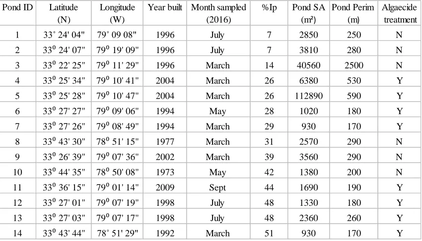
Table 2.1 General characteristics of each pond sampled
Pond ID Latitude Longitude Year built Month sampled %Ip Pond SA Pond Perim Algaecide
(N) (W) (2016) (m²) (m) treatment
1 33˚ 24' 04" 79˚ 09 08" 1996 July 7 2850 250 N 2 33⁰ 24' 07" 79⁰ 19' 09" 1996 July 7 3810 280 N 3 33⁰ 22' 25" 79⁰ 11' 29" 1996 March 14 40560 2500 N 4 33⁰ 25' 34" 79⁰ 10' 41" 2004 March 26 6380 530 Y 5 33⁰ 25' 28" 79⁰ 10' 47" 2004 March 26 112890 590 Y 6 33⁰ 27' 27" 79⁰ 09' 06" 1994 May 28 1020 180 Y
15
Chapter 3. Results
Sediment accumulation and bulk density
Sediment thickness was highly variable within each pond generally spanning 1 to
2 orders of magnitude. Interpolated maps of sediment thickness, however, allowed for a
mean sediment thickness to be determined in ponds with variable sediment thickness and
accumulation patterns. Some sample ponds experienced an even gradient of
sedimentation radiating from pond influent points (Figure 3.1 A), while others exhibited a
patchy pattern of accumulation, not necessarily reflective of pond morphology (Figure
3.1 B). Mean sediment thickness varied between ponds and ranged from 1.2 ± 0.1 to 20.5
± 0.8 cm. Using the sediment volume and bathymetric volumes calculated from
interpolation models, it was found that pond volume loss ranged from 1.0 ± 0.2 to 17.5 ±
0.5% (Table 3.1). Sediment accumulation rates ranged from 0.06 ± 0.01 to 0.50 ± 0.03
cm y-1 with a mean accumulation rate across all ponds of 0.32 ± 0.16 cm y-1 (Table 3.1).
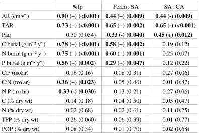
Sediment accumulation rate was directly correlated to catchment %Ip (R2 = 0.90, Figure
3.2), PA, and the PA:CA ratio (Table 3.1). There was no relationship between sediment accumulation rate and volume loss or pond age. Sediment bulk density varied with a
16
N-alkane Biomarkers
Reported alkane chain lengths ranged from C17 to C32 and generally showed a
bimodal distribution with peaks at C17 and C29. The mean chain length was 26 ± 1.9,
indicating a greater abundance of long chain n-alkanes. Total n-alkanes richness, the
amount of n-alkanes relative to total C was variable (median: 211, range: 19.2 ± 4.4 to
645 ± 306 μg g-1 C), however it was significantly correlated to %Ip (R2 = 0.57, p =
0.002). This positive relationship was driven by the long chain lengths n-alkanes; the
richness of C29 + C31 ranged from 6.2 ± 0.01 to 247 ± 117 μg g-1 C, with a median of 76.7
μg g-1 C (long chain n-alkanes versus %Ip R2 = 0.52, p = 0.004). In contrast, there was no
significant relationship between short chain n-alkane richness and %Ip (R2 = 0.04, p =
0.45). The richness of short chain n-alkanes (C17 + C19) was generally much lower ,
ranging from 4.1 ± 2.3 to 123 ± 38 μg g-1 C, with a median of 18.2 ± 29.5 μg g-1 C. One
pond, Sum, was an outlier with short length n-alkane richness of 123 ± 38 μg g-1 C, 3
times higher than the next closest pond, and 3.3 standard deviations above the mean. This
was the only pond that contains a significant pond sediment algal biomass signal. The
pond was also anomalous in that poor landscaping within its catchments has left bare
sandy soils, which seems to have resulted in high loading of mineral constituents to
sediments. It was hypothesized that these mineral constituents were driving sediment
accumulation and burying algal biomass before it can be mineralized at the sediment
surface interface. As such, this pond was removed from Index regression analyses.
TARHC ranged from 0.73 ± 0.01 to 12.6 ± 2.4, with a mean of 7.0 ± 4.3, while Paq
17
TARHC values > 1 and Paq values < 0.5 indicate that long chain n-alkanes dominate in
both indices. TARHC had a significant positive correlation with %Ip, perimeter:PA, and
AR, and negative a correlation with PA:CA (Table 3.2, Figure 3.3). TARHC had no
correlation with TPP (R2= 0.28, p = 0.07). P
aq had a negative correlation with perimeter :
PA, AR, and TPP (R2= 0.35, p = 0.034)., while it was positively correlated with SA: CA
(Table 3.2). Algaecide treatment appeared to have no effect on either biomass source
proxy.
Sediment nutrient composition
Mean sediment C, N, and P concentrations (mmol g-1) were determined for each
pond (Table 3.1). Pond sediment C concentrations varied from 6.84 to 21.5 % dry wt
with a mean concentration across all ponds of 12.0 ± 3.9 % dry wt (Table 3.2). Individual
pond N concentrations ranged from 0.408 to 1.26 % dry wt, and mean of 0.634 ± 0.227 %
dry wt across all ponds (Table 3.1). TPP concentrations varied from 0.080 to 0.344 %
dry wt with a mean of 0.190 ± 0.087 % dry wt across all ponds (Table 3.2). PIP
represented 68 ± 9% of the total P pool. PIP values ranged from 0.037 to 0.244 % dry wt
with a mean of 0.130 ± 0.061 % dry wt. POP varied from 0.035 to 0.139 % dry wt with a
mean of 0.058 ±0.029 % dry wt (Table 3.1). The variability of C and nutrient
concentrations across ponds was independent of catchment %Ip, perimeter:SA ratio, or
PA/CA ratio (Table 3.3). Sediment nutrient concentration measured on a per unit volume
scale, taking into account bulk density, showed slightly less variability. Mean C was 24.3
± 6.16 g cm-3 (range 14.1 – 31.6 g cm-3), N was 1.2 ± 0.24 g cm-3 (range 0.75 – 1.6 g cm
18
Sediment depth profiles revealed variable patters of down core nutrient
distribution (Figure 3.1). Significant negative correlations were found for C and N versus
depth in 27 of 29 cores (p < 0.05). Single sample t-tests rejected the null hypothesis that
regression slopes were equal to zero (C, p < 0.001); N, p < 0.001). Depth profiles further
showed N declines more rapidly than C, which was further confirmed by a matched pairs
t-test of the two slopes (p < 0.001). TPP, PIP, and POP versus depth profiles showed
greater variability relative to that of C and N. Of the 28 cores sampled for TPP, 10 had
significant negative correlations (p-values < 0.05), 3 had significant positive correlations
(p < 0.05), and the remainder had no significant correlation (p > 0.05). A single sample
t-test failed to reject the null hypothesis that slopes of TPP versus depth were equal to zero
(p = 0.064). For PIP, 6 had significant negative correlations (p < 0.05), 7 had significant
positive correlations (p < 0.05), and the remainder had no significant correlation (p >
0.05). A single sample t-test failed to reject the null hypothesis that slopes of PIP versus
depth were equal to zero (p = 0.66). POP values generally had greater errors than TPP,
PIP, C, or N as POP was calculated as the difference of TPP and PIP (difference between
two large numbers). For POP, 10 had significant negative correlations (p < 0.05), 4 had
significant positive correlations (p < 0.05), and the remainder hadno significant
correlation (p > 0.05). A single sample t-test failed to reject the null hypothesis that
slopes of POP versus depth were equal to zero (p = 0.81).
Sediment stoichiometric ratios showed a 2 to 4 fold variability between ponds
(Table 3.4). The mean of molar C:P ratio was 184 (range 91.9 – 377), C:N ratio was 24.3
(16.4 - 32.6), N:TPP ratio was 8.7 (4.3 – 19.0), and N:POP ratio is 26.0 (13.1 – 44.8).
19
(Table 3.4). The C:N ratio calculated from the slope of the regression between C and N of
all sections is 15.3 (R2 = 0.84, n = 417). The ratio of C:TPP showed no correlation with
any of the morphometric variables, while C:N is directly correlated with catchment %Ip,
and N:TPP was inversely correlated to %Ip (Table 3.3). These correlations were largely
driven by changes in C and P concentrations.
Burial rates of C, N, and P spaned more than an order of magnitude across all
ponds (Table 3.4). Mean C burial was 80 ± 44 g m-2 y-1 (range 8.7 to 161 g m-2 y-1). Mean
nitrogen burial was 3.73 ± 1.77 g m-2 y-1 (range 0.65 to 6.43 g m-2 y-1). Mean TPP burial
was 1.61 ± 1.07 g m-2 y-1 (range 0.238 to 4.13 g m-2 y-1). All nutrient burial rates were
directly correlated with both catchment % impervious surface and perimeter : SA(Table
20
Table 3.1 Sediment accumulation rates (AR), bulk density, and biomarker index results (TARHC and Paq).
Pond ID
1 50 ± 5.8 1.5% ± 0.2% 0.088 ± 0.01 0.39 ± 0.06 2.4 ± 1.2 0.23 ± 0.07
2 47 ± 7.7 1.0% ± 0.2% 0.062 ± 0.01 0.51 ± 0.12 1.0 ± 0.1 0.43 ± 0.06
3 1613 ± 91 ± 0.20 ± 0.02 0.30 ± 0.11 3.0 ± 0.1 0.30 ± 0.08
4 201 ± 14 ± 0.26 ± 0.03 0.32 ± 0.07 4.6 ± 3.0 0.33 ± 0.01
5 168 ± 23 ± 0.12 ± 0.02 0.29 ± 0.09 2.6 ± 2.0 0.49 ± 0.02
6 67 ± 2.1 9.1% ± 0.3% 0.30 ± 0.02 0.27 ± 0.03 9.4 ± 2.7 0.24 ± 0.03
7 70 ± 2.0 15.2% ± 0.4% 0.34 ± 0.02 0.40 ± 0.04 10.8 ± 5.2 0.19 ± 0.02
8 333 ± 27 10.1% ± 0.8% 0.33 ± 0.03 0.14 ± 0.01 7.9 ± 1.9 0.14 ± 0.09
9 206 ± 7.2 5.0% ± 0.2% 0.41 ± 0.03 0.34 ± 0.14 11.2 ± 1.8 0.17 ± 0.01
10 283 ± 8.1 17.5% ± 0.5% 0.48 ± 0.02 0.20 ± 0.02 6.1 ± 0.8 0.24 ± 0.03
11 63 ± 5.8 3.1% ± 0.3% 0.50 ± 0.08 0.29 ± 0.02 0.7 ± 0.1 0.43 ± 0.06
12 113 ± 3.7 6.6% ± 0.2% 0.47 ± 0.03 0.30 ± 0.09 12.6 ± 2.4 0.14 ± 0.03
13 214 ± 5.5 5.5% ± 0.1% 0.50 ± 0.03 0.38 ± 0.07 11.6 ± 6.8 0.22 ± 0.07
14 111 ± 1.9 14.2% ± 0.2% 0.50 ± 0.03 0.30 ± 0.07 11.3 ± 0.9 0.21 ± 0.01
Mean Median St dev Bulk Density (g cm¯³) 0.32 0.30 0.09 Biomarker indicies (cm y¯) % Filled Sed Vol (m³)
AR TARHC Paq
253 387 8.1% 5.4% 0.33 0.15 6.8 4.2 0.27 0.11
21
Table 3.2Carbon and nutrient characteristics of sediments.
Pond ID
1 11.2 ± 2.74 0.68 ± 0.12 0.174 ± 0.057 0.046 ± 0.003 0.109 ± 0.042 29.9 ± 11.8 1.6 ± 0.51 0.896 ± 0.584
2 6.84 ± 2.02 0.49 ± 0.14 0.087 ± 0.005 0.050 ± 0.004 0.037 ± 0.005 14.1 ± 3.9 1.0 ± 0.34 0.386 ± 0.124
3 11.6 ± 1.11 0.71 ± 0.11 0.080 ± 0.009 0.035 ± 0.008 0.049 ± 0.009 26.7 ± 5.4 1.4 ± 0.09 0.200 ± 0.046
4 10.7 ± 1.75 0.59 ± 0.05 0.204 ± 0.036 0.058 ± 0.010 0.145 ± 0.044 25.9 ± 4.0 1.3 ± 0.33 0.557 ± 0.089
5 12.1 ± 1.80 0.40 ± 0.04 0.127 ± 0.004 0.037 ± 0.012 0.101 ± 0.008 29.2 ± 4.2 1.1 ± 0.12 0.363 ± 0.078
6 7.29 ± 1.44 0.46 ± 0.06 0.121 ± 0.003 0.037 ± 0.005 0.084 ± 0.001 14.4 ± 2.3 0.87 ± 0.10 0.308 ± 0.029
7 8.93 ± 1.01 0.45 ± 0.05 0.152 ± 0.015 0.046 ± 0.013 0.114 ± 0.006 28.4 ± 1.0 1.3 ± 0.12 0.642 ± 0.079
8 21.5 ± 3.11 1.26 ± 0.14 0.318 ± 0.003 0.139 ± 0.007 0.183 ± 0.009 26.2 ± 0.7 1.5 ± 0.02 0.409 ± 0.038
9 10.4 ± 2.38 0.45 ± 0.19 0.227 ± 0.021 0.049 ± 0.018 0.155 ± 0.052 15.3 ± 5.3 0.75 ± 0.30 0.453 ± 0.182
10 16.5 ± 0.78 0.91 ± 0.06 0.323 ± 0.024 0.094 ± 0.004 0.234 ± 0.032 23.9 ± 0.9 1.1 ± 0.04 0.611 ± 0.109
11 6.98 ± 0.17 0.41 ± 0.02 0.083 ± 0.004 0.026 ± 0.002 0.067 ± 0.005 17.5 ± 1.6 0.90 ± 0.07 0.226 ± 0.020
12 15.2 ± 1.62 0.74 ± 0.11 0.230 ± 0.025 0.066 ± 0.006 0.166 ± 0.029 31.6 ± 5.4 1.3 ± 0.16 0.570 ± 0.112
13 13.4 ± 0.27 0.59 ± 0.04 0.344 ± 0.097 0.085 ± 0.009 0.244 ± 0.081 25.3 ± 3.1 0.99 ± 0.03 0.820 ± 0.353
14 15.0 ± 2.34 0.72 ± 0.10 0.184 ± 0.051 0.049 ± 0.008 0.129 ± 0.046 32.4 ± 3.7 1.3 ± 0.07 0.405 ± 0.165
Mean Median
St dev 6.16 0.24 0.198
24.3 1.2 0.489
(g cm¯³) (g cm¯³) (g cm¯³)
C N TPP
Sediment characteristics
(% dry wt) (% dry wt) (% dry wt) (% dry wt)
PIP POP
C N TPP
(% dry wt)
12.0 3.96 0.63 0.23 0.190 0.087 0.130 0.061 0.058 0.049 0.029
22
Table 3.3R2 and p values for simple linear regressions between various sediment and morphometric variables.
AR (cm y¯) 0.90 (+) (<0.001) 0.44 (+) (0.009) 0.44 (-) (0.009)
TAR 0.73 (+) (<0.001) 0.65 (+) (0.002) 0.65 (-) (<0.001)
Paq 0.30 (0.054) 0.33 (-) (0.040) 0.45 (+) (0.012)
C burial (g m¯² y¯) 0.78 (+) (<0.001) 0.58 (+) (0.002) 0.19 (0.12)
N burial (g m¯² y¯) 0.75 (+) (<0.001) 0.60 (+) (0.001) 0.25 (0.07)
P burial (g m¯² y¯) 0.56 (+) (0.002) 0.29 (+) (0.047) 0.12 (0.22)
C:P (molar) 0.16 (0.16) 0.08 (0.31) 0.27 (0.06)
C:N (molar) 0.36 (+) (0.023) 0.05 (0.46) 0.01 (0.87)
N:P (molar) 0.33 (-) (0.030) 0.13 (0.21) 0.27 (0.06)
C (% dry wt) 0.14 (0.18) 0.04 (0.50) 0.05 (0.47)
N (% dry wt) 0.02 (0.68) 0.02 (0.61) 0.11 (0.25)
TPP (% dry wt) 0.26 (0.060) 0.06 (0.39) 0.01 (0.77)
POP (% dry wt) 0.08 (0.34) 0.01 (0.70) 0.02 (0.68)
23
Table 3.4 Sediment stoichiometric ratios and C and nutrient burial rates.
Pond ID
1 230 ± 53 20.2 ± 2.5 12.1 ± 1.9 32.2 ± 6.6 26.2 ± 10.4 1.4 ± 0.4 0.787 ± 0.51
2 167 ± 68 16.4 ± 1.1 10.3 ± 3.9 19.8 ± 8.9 8.7 ± 2.4 0.65 ± 0.2 0.238 ± 0.08
3 377 ± 8 22.3 ± 3.6 19.0 ± 1.7 44.8 ± 7.3 53.2 ± 10.7 2.8 ± 0.2 0.398 ± 0.09
4 140 ± 8 27.3 ± 4.4 7.1 ± 0.9 30.3 ± 7.2 68.0 ± 10.4 3.3 ± 0.9 1.46 ± 0.23
5 215 ± 36 30.5 ± 3.1 7.3 ± 0.5 26.1 ± 1.0 36.2 ± 5.3 1.4 ± 0.2 0.450 ± 0.10
6 160 ± 31 18.9 ± 1.2 8.6 ± 1.5 21.6 ± 2.2 43.3 ± 6.8 2.6 ± 0.3 0.92 ± 0.09
7 137 ± 5 25.6 ± 0.5 5.9 ± 0.1 21.9 ± 2.3 97.1 ± 3.4 4.5 ± 0.4 2.19 ± 0.27
8 200 ± 11 21.5 ± 1.0 10.5 ± 0.5 26.0 ± 5.7 86.8 ± 2.4 4.9 ± 0.1 1.36 ± 0.12
9 92 ± 22 23.6 ± 1.9 4.3 ± 1.4 13.1 ± 8.3 63.4 ± 22.0 3.1 ± 1.2 1.87 ± 0.75
10 134 ± 13 23.6 ± 1.2 6.5 ± 0.8 23.4 ± 2.0 114 ± 4.4 5.5 ± 0.2 2.90 ± 0.52
11 201 ± 18 22.1 ± 0.5 9.4 ± 0.8 28.4 ± 1.8 87.0 ± 7.8 4.4 ± 0.4 1.12 ± 0.10
12 178 ± 4 27.3 ± 2.5 7.1 ± 0.5 27.8 ± 8.1 149 ± 25.6 6.3 ± 0.7 2.68 ± 0.53
13 135 ± 47 32.6 ± 2.8 5.3 ± 2.0 17.3 ± 2.9 128 ± 15.4 5.0 ± 0.1 4.13 ± 1.78
14 209 ± 25 28.5 ± 2.3 8.5 ± 1.1 32.0 ± 5.5 161 ± 18.5 6.4 ± 0.3 2.02 ± 0.82
Mean
Median
St dev
(molar) (molar) (molar)
C:P C:N
(molar) (g m¯² y¯) (g m¯² y¯) (g m¯² y¯)
TPP C N N:POP N:TPP 3.5 77.4 26.0 7.5 80.1 44.3 172 Burial rates Stoichiometric Ratios 1.41 1.61 1.07
23.6 7.9 26.0
24
Figure 3.1 Maps of sediment thickness from two example ponds. Color scale depicts sediment thickness, ranging from 2 to 18 cm. A) Pond 14 B) Pond 13
A
25
Figure 3.2 Simple linear regression between pond sediment accumulation rate and catchment %Ip. The regression is significant (p < 0.001, y = 1.03x – 0.003).
R² = 0.90
0 0.1 0.2 0.3 0.4 0.5 0.6 0.7
0% 10% 20% 30% 40% 50% 60%
M
e
an
A
R
(c
m
y
-1)
26
Figure 3.3 Linear regression between sediment accumulation rate and TARHC. Correlation is significant (p < 0.001), y = 24x - 0.13.
R² = 0.77
0 2 4 6 8 10 12 14 16 18 20
0 0.1 0.2 0.3 0.4 0.5 0.6 0.7
TA
RHC
27
Chapter 4. Discussion
Sediment accumulation rates were low, predicted by level of development
The State of South Carolina mandates the implementation and maintenance of
stormwater control structures for many coastal developments. These control structures
often take the form of stormwater wet detention ponds and are employed to mediate
flooding and to a secondary extent, reduce inputs of carbon, nutrient, and other
contaminants into local rivers, streams, and coastal oceans (SCDHEC 2005). The State
requires communities to dredge stormwater ponds when sediment accumulation displaces
25% of initial pond volume in order to effectively contain runoff (SCDHEC 2005). It has
therefore been argued that coastal ponds should be dredged every 5 to 10 years. Here we
show that, regardless of pond morphology and development intensity, coastal storm water
ponds have much lower sedimentation rates than previously anticipated by SCDHEC
(Table 3.1). Our estimates predicted it will take a median of 68 y (range 36.3 – 515 y) for
the stormwater ponds to reach the 25% water volume displacement limit. These
accumulation rates (Table 3.1) were significantly lower than those reported in agricultural
impoundments (mean 5.9 cm y-1, Downing et al., 2008), but were comparable to 10
Pennsylvania stormwater ponds albeit they are very different systems (range 0.06 – 0.53
28
The major predictor of sedimentation rate was not herbicide treatment or pond
morphology, but rather the relative percentage of impervious surfaces, such as roads,
parking lots, and buildings surrounding the pond. The strong relationship between
sedimentation rate and impervious surfaces (%Ip ,R2 = 0.90, Figure 3.1) thus serves as a
powerful tool for predicting pond infill rates and provides coastal communities with a
method for managing stormwater detention pond effectiveness. The relative distribution
of impervious surfaces is easily determined for most coastal communities using widely
available and free software, such as Google Earth or Google Earth Professional as
detailed within the methods section. Provided the relationship between sedimentation
rate and impervious surfaces holds true for ponds in similar settings to those in this study,
communities may be able to estimate sedimentation rates using Google Earth rather than
directly collecting sediments.
Terrestrial biomass drives sediment accumulation
Given previous studies in lakes and reservoirs, it was hypothesized that internal
algal production would be the major source of organic matter to sediments (Downing et al., 2008; Anderson et al., 2014). However, multiple indices showed that terrestrial biomass was the dominant source of sediment organic matter to SC coastal stormwater
ponds. Sediment surface C:N ratios were consistently greater than 10 (averaging 18.2 ±
2.8), indicating that pond sediments stored more terrestrial than algal biomass (Meyers
and Ishiwatari 1993). Additionally, both biomarker indices (Table 3.1) showed that
terrestrial signatures were significantly stronger than algal or aquatic macrophyte signals
29
study, 7.0, shows a significantly greater terrestrial signature than values reported in the
North American Great Lakes (median ~1.5) (Bourbonniere and Meyers 1996; Silliman et al., 1996; Meyers 1997; Lu and Meyers 2009) though a significantly lower terrestrial signature than found in Russian rivers (range 17 – 80) (van Dongen et al., 2008). Although TARHC does not provide absolute ratios of biomass, this index has been very
useful for comparing relative changes through time or across features in an ecosystem
(Bourbonniere and Meyers 1996) (van Dongen et al., 2008). In this study, the direct correlation between TARHC and accumulation rate indicates that the greatest terrestrial
signatures were observed in ponds with the greatest rates of sediment accumulation,
again suggesting that terrestrial biomass drives sediment accumulation (Figure 3.1). We
hypothesize that the dominance of terrestrial biomass in stormwater pond sediments is the
result of high loading of terrestrial biomass and low rates of algal biomass burial.
Addressing the sources of terrestrial matter, just as the amount of impervious
surface drove sedimentation rates (Fig 2), the proportion of terrestrial material was also
strongly positively correlated to the amount of impervious surfaces. It may seem
counterintuitive that ponds from catchments with the most impervious surfaces, and
therefore least total terrestrial biomass (e.g., trees, etc.), had the greatest amount of
sediment from terrestrial material (Table 3.2). We hypothesize that impervious surfaces
provide an important mechanism for the rapid transport of terrestrial material to
stormwater detention ponds from their catchments. In the South Carolina coastal plain,
runoff from urban watersheds was found to have ~ 5 times greater volume and to carry ~
5 times more suspended solids than runoff from forested watersheds (Corbett et al.,
30
runoff velocities required to transport biomass to the pond. The higher runoff velocities
from more developed catchments were more capable of transporting organic matter into
ponds either as sheet flow over lawns or as channeled through storm drains (Jacobson
2011). Here, it is important to note that impervious surface coverage never exceeded ~
50%. Thus, at least half of each pond’s catchment was open space, often taking the form
of well landscaped and maintained lawns. These lawns produced of large quantities of
easily transported grass clippings, providing a great source of external, terrestrial,
biomass to detention ponds. Ultimately the impacts of human development could increase
the export of terrestrial biomass to receiving waters, but high terrestrial loading alone
does not account for the observed low algal signature.
Algal blooms were observed in our stormwater ponds at the time of sampling and
have also been documented previously in South Carolina stormwater ponds (Siegel et al.,
2011; Reed et al., 2015). Our results indicate that, in spite of this internal production of algae, algal biomass is not ultimately being stored in pond sediment. Therefore the algal
biomass must have an alternate fate, which could be either direct export though weir
structures or remineralization. Pond volumes are designed such that they are well flushed
during rain events, potentially removing suspended algal biomass (SCDHEC 2005).
Additionally, algal biomass is thought to be more labile than terrestrial biomass and
undergoes preferential microbial remineralization (Zehnder and Svensson 1986;
Bastviken et al., 2004). This study did show clear signs of organic matter mineralization processes occurring in buried sediments. There was a universal decline of C and N
concentrations with depth, which is expected as over time, biomass is mineralized to
31
most the most time for mineralization processes to occur. N concentrations decreased
more rapidly with depth than did C, which suggests preferential remineralization of N
rich compounds (Benner 1991; Hopkinson et al., 1997). TPP did not exhibit uniform patterns of decline. A possible explanation of this pattern is the particle reactive nature of
the PO4-3 ion. As such, inorganic P remains in sediments after remineralization of
organic forms. POP did not consistently decline with increasing depth in pond sediments,
which could be a result of the high error inherent in the calculation of POP in PIP rich
systems.
A number of factors control microbial remineralization of C, and therefore the
missing algal biomass. Rates of microbial remineralization of organic C are controlled
by temperature and oxygen availability (Zehnder and Svensson 1986; Bastviken et al.,
2004; Gudasz et al., 2010). Large lakes and reservoirs commonly experience summer thermal stratification allowing hypolimnetic waters to remain between 4 – 10oC year
round and become seasonally anoxic (Boehrer and Schultze 2008). The small size and
shallow nature (1-3m) of South Carolina stormwater ponds prevent them from stratifying.
Their sediment water interfaces also thus experience mean summer temperatures as high
as 30oC and maintain near year round oxygen supply (Corbett et al., 1997; Serrano and DeLorenzo 2008). Therefore, it is quite possible that stormwater ponds experience
greater rates of microbial mineralization than larger lakes (Downing 2010). It is also
possible that the morphology of stormwater ponds increases their relative terrestrial load.
Their small size and generally irregular shape create large perimeter to surface area
32
terrestrial biomass inputs. Larger lakes have inherently lower perimeter to surface area
ratios reducing the potential load of terrestrial biomass per unit surface area.
Stormwater ponds are similar to natural lakes
Historically, stormwater ponds have been classified and studied as artificial water
bodies. However, the sediment nutrient dynamics of the stormwater ponds in this study
appear to be similar to those of natural lakes, and differ from other artificial waterbodies.
The carbon content of lake sediments was one parameter that differed from other
artificial water bodies. Mean pond sediment carbon concentration was 12% dry mass,
comparable to that found in natural lakes, yet about 3 – 4 fold greater than concentrations
reported in reservoir sediments (Table 4.1) (Brunskill et al., 1971; Gorham et al., 1974; Dean et al., 1993; Downing et al., 2008; Knoll et al., 2014). N and P concentrations follow a similar pattern, with pond sediment concentrations comparable to natural lakes
and slightly higher than reservoirs (Table 4.1) (Nürnberg 1988; Verstraeten and Poesen
2002; Gälman et al., 2008; Knoll et al., 2014). The high carbon richness in pond and lake sediments differences can likely be explained by patters of water flow management and
mineral sediment loading. Reservoirs and impoundments are dammed waterbodies with
continuous stream inputs, which may provide a means for greater transport of suspended
solids to basins. This increased load of mineral sediments will dilute the nutrient rich
organic sediments. The residential stormwater ponds sampled in this study only receive
inputs during rain events. Further, the communities within these ponds’ catchments have
careful landscaping and lawn care, reducing erosion and transport of mineral sediments.
The notable exception is the Sum pond community, where bare patches of lawn were
33
of 7.0% dry mass (Table 3.2), well below the all pond mean, suggesting greater mineral
loading relative to biomass loading.
Trends in pond nutrient burial also follow those observed in small natural lakes,
rather than those of reservoirs or impoundments. The mean C burial rate identified in this
study (80 g m-2 y-1, Table 3.4) is well within the range of mean burial rates reported in
literature for natural lakes, but 1 to 2 orders of magnitude below reported literature burial
rates of reservoirs (Table 4.1) (Mulholland and Elwood 1982; Höhener and Gächter
1993; Dean and Gorham 1998; Downing et al., 2008; Mackay et al., 2012; Knoll et al.,
2014). Direct measurements of N and P burial rates are rarely reported in literature.
However, this study’s mean N and P burial (N: 3.8 g m-2 y-1, P: 1.6 g m-2 y-1) were
comparable to those of European lakes and Green Bay, Lake Michigan, while still an
order of magnitude below reported reservoir burial rates (Table 4.1) (Höhener and
Gächter 1993; Klump et al., 1997; Mengis et al., 1997; Mackay et al., 2012; Knoll et al.,
2014). We hypothesize that the consistently higher burial rates of reservoirs is a result of
their hydrology. The constant inputs of suspended solids and nutrients via rivers or
streams to reservoirs leads to high rates of mass burial, which compensate for lower
nutrient concentrations and result in very high total burial rates. The ponds in this study,
as well as for many natural lakes, receive inputs more episodically and are often linked
with precipitation events. These periodic inputs likely result in less total mass loading and
ultimately lower carbon and nutrient burial rates. This study’s rates of nitrogen burial are
also significantly lower than published rates of denitrification in stormwater retention
ponds (1.6 – 21 g m-2 y-1), therefore looking at sediment burial rates of N alone likely
34
Stormwater ponds as novel sinks in the urban hydrology
In urban systems many of the drivers of biogeochemical cycles are controlled by
humans, for example impervious surface coverage and excess loading of nutrients from
waste, fertilizer, and detergents (Kaye et al., 2006). These anthropogenic impacts can
alter local hydrology, degrading stream quality and increasing nutrient export to receiving
waters (Walsh et al., 2005; Booth et al., 2016). Stormwater ponds are ultimately designed
as engineering control measures to mitigate impacts of urbanization to local hydrology
and water quality. As ponds are designed to intentionally intercept sediment and nutrient
export via stormwater flows, ponds are hotspots of biogeochemical activity, where
nutrients can be passed between oxidation states, organic, and inorganic forms. Previous
studies have found that stormwater detention ponds provide variable, yet significant,
removal of nutrients and pollutants (Wu et al., 1996; Comings et al., 2000; Mallin et al.,
2002). These previous studies have focused on the mass balance of influent and effluent.
Our study addressed the removal of C and nutrient by quantifying the rate burial (change
of storage) directly.
A first-cut at estimating the regional significance of pond C and nutrient
sequestration rates can be made by scaling up results of this study to the total number of
ponds that exist in coastal South Carolina. A recent estimate of small artificial water
bodies in the eight coastal counties of South Carolina suggests there are more than 21,500
manmade ponds, representing a mix of rural, agricultural and development-related
stormwater ponds (E. Smith, unpublished data). Of this total, 9,269 ponds are associated
with coastal development, and 5,073 of these are associated with residential development
35
area of 25.3 km2. Assuming the mean burial rates observed in this study apply, just the
residential ponds alone (representing 24% of the total pond population) bury 2.0 x 10⁹ g
C y-1, 9.5 x10⁷ g N y-1, and 3.7 x10⁷ g P y-1. The proliferation of ponds along this
coastal zone thus represents a long-term storage of C, N and P that would otherwise have
been transported to coastal receiving waters. Stormwater pond sequestration values show
that these ponds serve as nontrivial C and nutrient sinks on the local and regional scale.
What remains unclear, however, is whether these rates of sequestration are ecologically
significant in the context of broader coastal eutrophication and climate change.
Stormwater ponds are a fixture of urban hydrology, experiencing great anthropogenic
nutrient loading, yet a full understanding of how these feature function in a complex
hydrology is understudied. Further work is thus necessary if we are to integrate these
small, but increasingly significant, ponds into a broader biogeochemical-hydrologic
36
Table 4.1 Comparison of sediment C, N, and P concentrations and burial rates between waterbodies in this study and others.
Source Description C N P C burial N burial TPP burial
(% dry wt) (% dry wt) (%dry wt) (g m¯² y¯) (g m¯² y¯) (g m¯² y¯)
This study Stormwater ponds† (14), SC 12 0.63 0.19 80 3.7 1.6
(6.8 – 22) (0.41 – 1.3) (0.080 - 0.34) (8.7 - 161) (0.65 – 6.4) (0.24 – 4.1)
Dean et al., 1993 Lakes* (46), Minnesota 12 72
(3 - 29)
Mulholland and Elwood 1982 Small Oligotrophic lakes* (14), USA 27
(3 - 128)
Mulholland and Elwood 1982 Small Meso-Eutrophic lakes* (18), USA 94
(11 - 198)
Höhener and Gächter 1993 Lakes* (10), EU 5.0 ± 1.6
Mackay et al., 2012 Lake* (1), UK 44.3
Mengis et al., 1997 Lakes* (2), Switzerland 0.29 3.6
(0.26 - 0.32) (3.1 – 4.1)
Klump et al., 1997 Green Bay, Lake Michigan* (1) 0.024 2
Gorham et al., 1974 Lakes* (20), UK 7
(4 - 13)
Brunskill et al., 1971 Lakes* (23), Wisconsin 20
Nürnberg 1988 Global mean P 0.3
Verstraeten and Poesen 2002 Agriculture ponds† (12), Belgium 0.085
(0.051 - 0.20)
Mulholland and Elwood 1982 Reservoirs† (24), USA 350
(52 - 2000)
Downing et al., 2008 Agricultural impoundments† (40), Iowa 4.8 2122
(148 - 17400)
Knoll et al., 2014 Reservoirs† (13), Ohio 2.3 0.32 0.1 246 33 13
37
Chapter 5. Conclusion
Stormwater ponds are designed to operate as part of an urban landscape, with
much of their function directly controlled by surrounding land use. Here, we find that
pond sediment accumulation rates are driven by terrestrial sources and are predicted by
the development intensity of their catchments in coastal South Carolina. The shallow
morphology of these ponds creates ideal conditions for rapid rates of microbial
remineralization, resulting in limited algal derived biomass accumulation. Although
driven by different processes, stormwater pond C and nutrient sediment composition and
burial are remarkably similar to those of natural lakes from across the world. The
biogeochemical consistency between pond and lake sediments suggests that, collectively,
ponds could play significant roles in global carbon and nutrient cycling. The scope of this
project was very narrow, limited to detention ponds in residential communities. To more
accurately extrapolate C and nutrient sequestration in small waterbodies it would be
valuable to identify burial rates associated with other land uses, such as commercial,
38
References
Anderson, N. J., H. Bennion and A. F. Lotter (2014). "Lake eutrophication and its
implications for organic carbon sequestration in Europe." Global Change Biology
20(9): 2741-2751.
Bastien, N. R. P., S. Arthur and M. J. McLoughlin (2012). "Valuing amenity: public perceptions of sustainable drainage systems ponds." Water and Environment Journal 26(1): 19-29.
Bastviken, D., L. Persson, G. Odham and L. Tranvik (2004). "Degradation of dissolved organic matter in oxic and anoxic lake water." Limnology and Oceanography
49(1): 109-116.
Benner, R. (1991). "Diagenesis of belowground biomass of Spartina alterniflora in saltmarsh sediments." Limnol. Oceanogr. 36: 1358-1374.
Biggs, J., P. Williams, M. Whitfield, P. Nicolet and A. Weatherby (2005). "15 years of pond assessment in Britain: results and lessons learned from the work of Pond Conservation." Aquatic Conservation: Marine and Freshwater Ecosystems 15(6): 693-714.
Bishop, C. A., J. Struger, L. J. Shirose, L. Dunn and G. D. Campbell (2000). "Contamination and wildlife communities in stormwater detention ponds in Guelph and the Greater Toronto Area, Ontario, 1997, and 1998. Part 2.
Contamination and biological effects of contamination." Water Quality Research Journal of Canada 35(3): 437-434.
Boehrer, B. and M. Schultze (2008). "Stratification of lakes." Reviews of Geophysics
46(2).
Bourbonniere, R. A. and P. A. Meyers (1996). "Sedimentary geolipid records of historical changes in the watersheds and productivities of Lakes Ontario and Erie." Limnology and Oceanography 41(2): 352-359.
Brunskill, G., D. Povoledo, B. Graham and M. Stainton (1971). "Chemistry of surface sediments of sixteen lakes in the Experimental Lakes Area, northwestern Ontario." Journal of the Fisheries Board of Canada 28(2): 277-294. Chiandet, A. S. and M. A. Xenopoulos (2011). "Landscape controls on seston
stoichiometry in urban stormwater management ponds." Freshwater Biology
56(3): 519-529.
Clow, D. W., S. M. Stackpoole, K. L. Verdin, D. E. Butman, Z. Zhu, D. P. Krabbenhoft and R. G. Striegl (2015). "Organic Carbon Burial in Lakes and Reservoirs of the Conterminous United States." Environmental Science & Technology 49(13): 7614-7622.
39
"Plumbing the Global Carbon Cycle: Integrating Inland Waters into the Terrestrial Carbon Budget." Ecosystems 10(1): 172-185.
Comings, K. J., D. B. Booth and R. R. Horner (2000). "Storm water pollutant removal by two wet ponds in Bellevue, Washington." Journal of Environmental Engineering
126(4): 321-330.
Corbett, C. W., M. Wahl, D. E. Porter, D. Edwards and C. Moise (1997). "Nonpoint source runoff modeling A comparison of a forested watershed and an urban watershed on the South Carolina coast." Journal of Experimental Marine Biology and Ecology 213(1): 133-149.
Corbett, D. R., W. C. Burnett, P. H. Cable and S. B. Clark (1997). "Radon tracing of groundwater input into Par Pond, Savannah River site." Journal of Hydrology
203(1-4): 209-227.
Dean, W. E. and E. Gorham (1998). "Magnitude and significance of carbon burial in lakes, reservoirs, and peatlands." Geology 26(6): 535-538.
Dean, W. E., E. Gorham and D. J. Swaine (1993). "Geochemistry of surface sediments of Minnesota lakes." Geological Society of America Special Papers 276: 115-134. Downing, J., Y. Prairie, J. Cole, C. Duarte, L. Tranvik, R. Striegl, W. McDowell, P.
Kortelainen, N. Caraco and J. Melack (2006). "The global abundance and size distribution of lakes, ponds, and impoundments." Limnology and Oceanography
51(5): 2388-2397.
Downing, J. A. (2010). "Emerging global role of small lakes and ponds." Limnetica
29(1): 0009-0024.
Downing, J. A., J. J. Cole, J. J. Middelburg, R. G. Striegl, C. M. Duarte, P. Kortelainen, Y. T. Prairie and K. A. Laube (2008). "Sediment organic carbon burial in agriculturally eutrophic impoundments over the last century." Global Biogeochemical Cycles 22(1): n/a-n/a.
Eglinton, G. and R. Hamilton (1967). "Leaf Epicuticular Waxes." AAAS: 1322-1335. Ficken, K. J., B. Li, D. L. Swain and G. Eglinton (2000). "An n-alkane proxy for the
sedimentary input of submerged/floating freshwater aquatic macrophytes." Organic Geochemistry 31(7-8): 745-749.
Gälman, V., J. Rydberg, S. S. de‐Luna, R. Bindler and I. Renberg (2008). "Carbon and nitrogen loss rates during aging of lake sediment: changes over 27 years studied in varved lake sediment." Limnology and Oceanography 53(3): 1076-1082. Gorham, E., J. W. Lund, J. E. Sanger and W. E. Dean (1974). "Some relationships
between algal standing crop, water chemistry, and sediment chemistry in the English Lakes."
40
Gudasz, C., D. Bastviken, K. Steger, K. Premke, S. Sobek and L. J. Tranvik (2010). "Temperature-controlled organic carbon mineralization in lake sediments." Nature
466(7305): 478-481.
Harrison, J. A., R. J. Maranger, R. B. Alexander, A. E. Giblin, P.-A. Jacinthe, E. Mayorga, S. P. Seitzinger, D. J. Sobota and W. M. Wollheim (2009). "The regional and global significance of nitrogen removal in lakes and reservoirs." Biogeochemistry 93(1): 143-157.
Höhener, P. and R. Gächter (1993). "Prediction of dissolved inorganic nitrogen (DIN) concentrations in deep, seasonally stratified lakes based on rates of DIN input and N removal processes." Aquatic Sciences-Research Across Boundaries 55(2): 112-131.
Holland, A. F., D. M. Sanger, C. P. Gawle, S. B. Lerberg, M. S. Santiago, G. H. Riekerk, L. E. Zimmerman and G. I. Scott (2004). "Linkages between tidal creek
ecosystems and the landscape and demographic attributes of their watersheds." Journal of Experimental Marine Biology and Ecology 298(2): 151-178.
Hopkinson, C. S., B. Fry and A. L. Nolin (1997). "Stoichiometry of dissolved organic matter dynamics on the continental shelf of the northeastern U.S.A." Continental Shelf Research 17(5): 473-489.
Jacobson, C. R. (2011). "Identification and quantification of the hydrological impacts of imperviousness in urban catchments: A review." Journal of Environmental Management 92(6): 1438-1448.
Klump, J. V., D. N. Edgington, P. E. Sager and D. M. Robertson (1997). "Sedimentary phosphorus cycling and a phosphorus mass balance for the Green Bay (Lake Michigan) ecosystem." Canadian Journal of Fisheries and Aquatic Sciences 54(1): 10-26.
Knoll, L. B., M. J. Vanni, W. H. Renwick and S. Kollie (2014). "Burial rates and
stoichiometry of sedimentary carbon, nitrogen and phosphorus in Midwestern US reservoirs." Freshwater Biology 59(11): 2342-2353.
Lu, Y. and P. A. Meyers (2009). "Sediment lipid biomarkers as recorders of the contamination and cultural eutrophication of Lake Erie, 1909–2003." Organic Geochemistry 40(8): 912-921.
Mackay, E. B., I. D. Jones, A. M. Folkard and P. Barker (2012). "Contribution of sediment focussing to heterogeneity of organic carbon and phosphorus burial in small lakes." Freshwater Biology 57(2): 290-304.
Mallin, M. A., S. H. Ensign, T. L. Wheeler and D. B. Mayes (2002). "Pollutant Removal Efficacy of Three Wet Detention Ponds." Journal of Environment Quality 31(2): 654.
41
Meyers, P. (2003). "Applications of organic geochemistry to paleolimnological
reconstructions: a summary of examples from the Laurentian Great Lakes." Org Geochem: 261-289.
Meyers, P. A. (1997). "Organic geochemical proxies of paleoceanographic,
paleolimnologic, and paleoclimatic processes." Organic Geochemistry 27(5-6): 213-250.
Meyers, P. A. and R. Ishiwatari (1993). "Lacustrine organic geochemistry—an overview of indicators of organic matter sources and diagenesis in lake sediments." Organic Geochemistry 20(7): 867-900.
Mulholland, P. J. and J. W. Elwood (1982). "The role of lake and reservoir sediments as sinks in the perturbed global carbon cycle." Tellus 34(5): 490-499.
Nürnberg, G. K. (1988). "Prediction of phosphorus release rates from total and reductant-soluble phosphorus in anoxic lake sediments." Canadian Journal of Fisheries and Aquatic Sciences 45(3): 453-462.
Reed, M. L., G. R. DiTullio, S. E. Kacenas and D. I. Greenfield (2015). "Effects of nitrogen and dissolved organic carbon on microplankton abundances in four coastal South Carolina (USA) systems." Aquatic Microbial Ecology 76(1): 1-14. Saunders, D. L. and J. Kalff (2001). Hydrobiologia 443(1/3): 205-212.
SCDHEC (2005). Storm Water Management BMP Handbook S. C. D. o. H. a. E. Control: 5-9 to 5-12.
Serrano, L. and M. E. DeLorenzo (2008). "Water quality and restoration in a coastal subdivision stormwater pond." Journal of Environmental Management 88(1): 43-52.
Siegel, A., B. Cotti-Rausch, D. I. Greenfield and J. L. Pinckney (2011). "Nutrient controls of planktonic cyanobacteria biomass in coastal stormwater detention ponds." Marine Ecology Progress Series 434: 15-27.
Silliman, J. E., P. A. Meyers and R. A. Bourbonniere (1996). "Record of postglacial organic matter delivery and burial in sediments of Lake Ontario." Organic Geochemistry 24(4): 463-472.
Smith, S. V., W. H. Renwick, J. D. Bartley and R. W. Buddemeier (2002). "Distribution and significance of small, artificial water bodies across the United States
landscape." Science of The Total Environment 299(1-3): 21-36.
Søndergaard, M., E. Jeppesen and J. P. Jensen (2005). "Pond or lake: does it make any difference?" Archiv für Hydrobiologie 162(2): 143-165.
Stankowski, S. J. (1972). "Population density as an indirect indicator of urban and suburban land-surface modifications." US Geological Survey Professional Paper
800: 219-224.
42
Tranvik, L. J., J. A. Downing, J. B. Cotner, S. A. Loiselle, R. G. Striegl, T. J. Ballatore, P. Dillon, K. Finlay, K. Fortino, L. B. Knoll, P. L. Kortelainen, T. Kutser, S. Larsen, I. Laurion, D. M. Leech, S. L. McCallister, D. M. McKnight, J. M. Melack, E. Overholt, J. A. Porter, Y. Prairie, W. H. Renwick, F. Roland, B. S. Sherman, D. W. Schindler, S. Sobek, A. Tremblay, M. J. Vanni, A. M. Verschoor, E. von Wachenfeldt and G. A. Weyhenmeyer (2009). "Lakes and reservoirs as regulators of carbon cycling and climate." Limnology and Oceanography
54(6part2): 2298-2314.
Tweel, A., E. M. Smith, D. M. Sanger and E. Koch (2016). A stormwater pond inventory for the eight coastal counties of South Carolina. SC Water Resources Conference. Columbia, SC.
van Dongen, B. E., I. Semiletov, J. W. H. Weijers and Ö. Gustafsson (2008).
"Contrasting lipid biomarker composition of terrestrial organic matter exported from across the Eurasian Arctic by the five great Russian Arctic rivers." Global Biogeochemical Cycles 22(1): n/a-n/a.
Verstraeten, G. and J. Poesen (2000). "Estimating trap efficiency of small reservoirs and ponds: methods and implications for the assessment of sediment yield." Progress in Physical Geography 24(2): 219-251.
Verstraeten, G. and J. Poesen (2002). "Regional scale variability in sediment and nutrient delivery from small agricultural watersheds." Journal of environmental quality
31(3): 870-879.
Weinstein, J. E., K. D. Crawford and T. R. Garner (2010). "Polycyclic aromatic hydrocarbon contamination in stormwater detention pond sediments in coastal South Carolina." Environmental monitoring and assessment 162(1): 21-35. Wu, J. S., R. E. Holman and J. R. Dorney (1996). "Systematic Evaluation of Pollutant
Removal by Urban Wet Detention Ponds." Journal of Environmental Engineering
122(11): 983-988.
Zehnder, A. J. B. and B. H. Svensson (1986). "Life without oxygen: what can and what cannot?" Experientia 42(11-12): 1197-1205.