Approximation algorithm for data broadcasting in duty cycled multi hop wireless networks

R E S E A R C H

Open Access

Approximation algorithm for data

broadcasting in duty cycled multi-hop wireless

networks

Dianbo Zhao

and Kwan-Wu Chin

Abstract

Broadcast is a fundamental operation in wireless networks. To this end, many past studies have studied the NP-hard, broadcast problem for always-on multi-hop networks. However, in wireless sensor networks, nodes are powered by batteries, meaning, they have finite energy. Consequently, nodes are required to have a low duty cycle, whereby they switch between active and sleep state periodically. This means that a transmission from a node may not reach all of its neighbors simultaneously. Consequently, any developed broadcast protocols must consider collisions and the wake-up times of neighboring nodes. Henceforth, this paper studies the minimum latency broadcast scheduling problem in duty cycled multi-hop wireless networks (MLBSDC), which remains NP hard. The MLBSDC problem aims to find a collision-free schedule that minimizes the time in which the last node receives a broadcast message. We propose a novel algorithm called CFBS that allows nodes in different layers of the broadcast tree to transmit simultaneously. We prove that CFBS produces a latency of at most(T+1)H+TO(log₂H). Here,Tdenotes the number of time slots in a scheduling period, andHis the optimal broadcast latency obtained from the shortest path tree algorithm assuming no collision. We also show that the total number of transmissions is at most 4(T+2)times larger than the optimal value. The results from extensive simulation show that CFBS has a better performance than OTAB, the best broadcast scheduling algorithm to date. In particular, the broadcast latency achieved by CFBS is up to₂₀3 that of OTAB.

1 Introduction

Wireless sensor networks (WSNs) consist of numerous sensor nodes deployed in a field. These nodes are usu-ally resource constrained in terms of battery lifetime and computation, and are equipped with a number of sens-ing elements. Moreover, they have one or more radios and communicate with each other via multi-hop communi-cations because these radios have a bounded and short transmission range. In addition, there exist one or more sinks to collect sensed data and to issue commands that affect the operation of sensor nodes. To date, WSNs have found a myriad of applications. For example, precision agriculture [1], monitoring of pests [2], and volcanology [3] to name a few.

Network-wide broadcast is a fundamental operation in wireless networks, where a message needs to be prop-agated from a source node, e.g., a sink, to all other

*Correspondence: [email protected]

School of Electrical, Computer & Telecommunications Engineering, University of Wollongong, Wollongong, 2500, Australia

nodes. It is relied upon by several network protocols, such as routing [4], information dissemination [5], and resource/services discovery [6]. These protocols in turn help applications in disaster relief, military communi-cation, rescue operation, and object detection [7]. For these applications, time is critical, and hence, a minimum latency broadcast scheduling (MLBS) algorithm/protocol will be of great importance to their operation. Like many other communication protocols, any developed MLBS solution must deal with collision. Unfortunately, the MLBS problem for multi-hop wireless networks has been proven to be NP hard [8], and researchers have proposed many approximation algorithms. These algo-rithms, however, assume that all nodes are always active. They typically make use of neighborhood information to determine whether a node needs to transmit a message. Specifically, collisions can be detected by identifying the common neighbors of two or more transmitting nodes via topological information and ensuring the interfering nodes transmit in different time slots.

In contrast, the MLBS problem is quite different in duty cycled WSNs. Briefly, in these networks, nodes are pow-ered by batteries and are only awake for a fraction of the time [9]. Here, the duty cycle of a node is defined as the ratio between its active time and the scheduling period, i.e., T. We note that WSNs can employ a synchronous wake-up schedule, that is, nodes wake up at the same time. However, nodes will have to coordinate and synchronize their wake-up time globally and, hence, incur high signal-ing overheads. This paper, therefore, only considers WSNs with asynchronous schedule, where nodes determine their wake-up time independently and randomly.

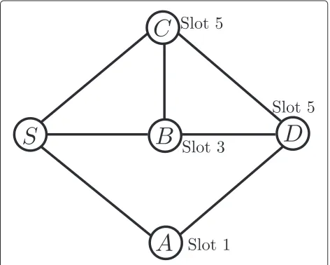
As an example, consider Figure 1. Node S needs to broadcast a message to nodesA,B,C, andD. All of which have different wake-up times, i.e., time slot ‘1’, ‘3’, ‘5’, and ‘5’, respectively. Here, nodeS may transmit the message at least three times because its neighbors A, B, and C have different wake-up times. Moreover, assuming node A has received the message from s at time slot ‘1’ and Breceived the message from Sat time slot ‘3’, nodesS, A, andBmay try to forward the message to their neigh-bors at time slot ‘5’. However, this will cause a collision at nodes C and D. Considering the fact thatB is adja-cent to nodesCandD, both with the same wake-up time of ‘5’, one feasible way to conduct the broadcast is for S to send the message to A and B at time slot ‘1’ and ‘3’, respectively, after whichBtransmits it toCandDat time slot ‘5’. As we can see, both topology and wake-up schedule of nodes are key issues to consider when solving the MLBSDC problem. In fact, this consideration ren-ders the MLBS problem more complex, meaning, existing algorithms for always-on wireless networks are no longer applicable.

Henceforth, this paper presents the design and evaluation of a novel approximation algorithm that has

Figure 1Broadcast in duty cycled WSNs.

significantly better performance than prior solutions. Specifically, it contains the following contributions:

1. A novel algorithm called centralized collision-free broadcast scheduling (CFBS) that is suitable for both always-on and duty cycled networks. CFBS produces a broadcast latency of at most

(T+1)H+TO(log₂H), where the constant before TO(log₂H)does not exceed 108. In particular, for always-on networks, i.e.,T =1, the broadcast latency of CFBS is bounded by2R+O(log₂R), whereR is the maximum hop distance from the source to any node. 2. The total number of transmissions produced by

CFBS is at most4(T+2)times that of the minimum total number of transmissions. For always-on networks, this approximation ratio is 12. 3. We evaluate CFBS under different network

parameters via simulation and show that that on average, our proposed algorithm has a much better performance in terms of broadcast latency than the state of the art algorithm OTAB [10]. The key reason is our algorithm is able to schedule transmissions in multiple layers as opposed to layer by layer, as is done by OTAB. Moreover, it allows non-interfering nodes in lower layers to transmit even though nodes in the current layer have not finished their transmission.

2 Related works

To date, there are many approaches to carry out broad-cast in multi-hop wireless networks. The simplest by far is flooding [11], where each node simply re-transmits a received message to its neighbors unscrupulously. How-ever, this causes broadcast storms [12] and is thus very costly and causes long latencies. Consequently, a num-ber of researchers, e.g., [13-15], have proposed methods that improve the efficiency of broadcast. In this paper, we address a variant of the MLBS problem, which aims to find an efficient, collision-free schedule that yields the minimum broadcast latency.

Gandhi et al. [8] presented an approximation algorithm with a constant approximation ratio of more than 400 for one-to-all broadcast. They then improve this ratio to 12 in [7]. Huang et al. [16] outlined three approximation algo-rithms for MLBS with latency of at most 24R, 16R, and R+O(log₂R), respectively, and the omitted constant in

O(log₂R)exceeds 150 [7].

In particular, the two methods proposed in [19] have an approximation ratio of 3(ln+ 1) and 20 in terms of the number of transmissions, respectively, whereis the maximum degree. These works, however, have not addressed the MLBSDC problem in duty cycled networks. To date, there are only a handful of directly related works. Hong et al. [20] proved that the MLBSDC problem is NP hard and proposed two approximation algorithms: SLAC and ELAC. Their algorithms achieve an approxima-tion ratio ofO((2+1)T)and 24T+1, respectively, where is the maximum degree, andT denotes the number of time slots in a scheduling period. Both algorithms apply the D2-coloring approach [21] to schedule transmissions on a shortest path tree. In [10], Jiao et al. show that ELAC can be improved further by using D2-coloring twice at each layer of the shortest path tree. They propose an algo-rithm called OTAB and prove that OTAB has an approx-imation ratio of 17T. Also, they showed that the total number of transmissions scheduled by OTAB is at most 15 times larger than the minimum number of transmis-sions. Duan et al. [22] provide a generalized algorithm for the MLBSDC problem with an approximation ratio ofT. They transform the MLBSDC problem into the conven-tional maximum independent set problem and try to find a maximum set of non-interfering senders in each time slot. Recently, Xu et al. [23] extended the pipelined broad-cast scheme in [16] to consider duty cycled WSNs. Their broadcast algorithm produces a latency of at mostTH+ TO(log₂H), where the omitted constant inTO(log₂H) also exceeds 150; in contrast, our solution has 108 as a constant inTO(log₂H).

The key limitation of [20] and [10] is that transmis-sions are scheduled layer by layer based on a shortest path tree, which prevent non-interfering nodes in lower layers from transmitting until all nodes in the current layer finish their transmissions. The broadcast latency performance of [22] is mainly influenced by the maximum degree of nodes, i.e.,, which produces a large bound for dense networks. Unlike [20] and [10], our proposed algorithm is able to schedule nodes’ transmissions in more than one layer, leading to a lower latency. The broadcast latency of CFBS is mainly influenced byH, which does not rely on the number of nodes or maximum degree. All these fea-tures constitute key advantages over [22] and also result in an algorithm that is suitable for dense networks.

3 Preliminaries 3.1 Network model

We consider a duty cycled WSN which has a schedul-ing period that is divided intoT slots of fixed and equal length, and is indexed by 0, 1, 2,· · ·,T−1. Each time slot is assumed to be of sufficient duration to receive a mes-sage. We assume that the network is locally synchronized at a slot level. As shown in [24], this can be achieved

using local synchronization techniques, such as Flood-ing Time Synchronization Protocol (FTSP) [25]. The duty cycle of a node is defined as _T1, where the numerator cor-responds to one active time slot. Similar to [10,20,26], each nodevselects to wake up at a time slot in the range [0, 1,· · ·,T−1] randomly and independently in order to receive a message. We will denote nodev’s wake-up slot asτ (v). If nodevwants to transmit a message, it will wake up at the corresponding receiver’s wake-up slot. Here, we assume there is no message or bit error, and links are bidi-rectional. This is reasonable because any retransmissions due to bit errors can be accounted for by dimensioning the slot size accordingly. However, a message is considered lost if there is a collision, i.e., two or more simultaneous transmissions to a common node. A node must not receive and send a message at the same time. We will useN(v)to denote the set of one-hop neighbors of nodev∈V, andn is the cardinality ofV, i.e.,n= |V|.

The duty cycled WSN is modeled as a weighted unit disc graph (UDG)G = (V,E), whereV is the set of nodes, andErepresents the set of edges/links that exist between two nodes if their Euclidean distance is no more than a given transmission range. Furthermore, each edge in V has an associated numerical value, called a weight or cost. This corresponds to the time interval between two nodes’ active time slots. Specifically, for each edge (u,v) ∈ E, itscost, denoted asedc(u,v), is defined as per Equation 1, wheresis the source node.

in an always-on network, which can be modeled by setting T =1, we have Rad(G,s)=R.

Anindependent set(IS)IofG(V,E)is defined as a sub-set ofV, such that ifu,v∈ I, then(u,v) /∈ E. Amaximal independent set (MIS)U is an independent set which is not a subset of any other independent sets. A subsetUof V is adominating set ofGif each node not inU is adja-cent to at least a member ofU. Clearly, every MIS ofGis also a dominating set ofG. If setUis a dominating set ofG andG[U] is connected, thenUis called aconnected dom-inating set (CDS) ofG. The authors of [27] showed that the MIS size of a UDG graph is bounded byO(R2). It is also known that the size of MIS does not exceed 4opt+1, whereoptdenotes the minimum size of a CDS ofG[28].

A proper D2-coloring [21] of G is an assignment of colors, labeled by natural numbers to the nodes in V, such that any pair of nodes within two-hop neighborhood receives different colors. Any node orderingv1,v2,· · ·,vn ofV induces a proper node coloring ofGin the first-fit manner. Specifically, fori=1 ton, assign nodevithe least assigned color that is not used by any neighborvj, where j<i. For example, consider a line topologyA−B−C. A proper coloring results in the color assignments 1, 2, and 1 to nodesA,B, andC, respectively. A particular node order-ing of interest is thesmallest-degree-last ordering[29]. For i = nto 1, it setsvi to the node with smallest degree in G[U], whereU ⊆V. Initially, setUtoV, and then repeat the following iteration untilUbecomes empty: fori = n to 1, setvito the node with the smallest degree inU, and remove it fromU. Consider the line topologyA−B−C. The smallest-degree-last ordering will be C−B−A. A summary of notations used in this paper can be found in Table 1.

3.3 Problem formulation

Our problem, called MLBSDC, concerns the broadcast of a message from a source nodes ∈ V to all other nodes. The goal is to minimize the time in which the last node receives the message. Without loss of generality, we define the start time of node s’s broadcast to be slot zero, and the broadcast latency is the maximum time taken by a message to reach all nodes.

We model the MLBSDC problem as follows. Let(Si,ti+ kiT)denote theith transmission, andi,ki ∈N. At theith transmission, the nodes in the setSitransmit the message to nodes inRiat timeti+kiT, whereRidenotes the set of nodes that received the message from nodes inSi colli-sion free, andtiis the active time slot of nodes inRi. The MLBSDC problem is then to find a forwarding schedule

S= {(s, 0),(S1,t1+k1T),· · ·,(Sm,tm+kmT)} (2)

that satisfies the following constraints: (1) t1 +k1T < t2+k2T < . . . < tm+kmT, (2) any node in Si cannot be scheduled to transmit the message until it receives the

Table 1 Commonly used notations

Notation Meaning

G(V,E) Network graph

N(v) v’s one-hop neighbors

T Scheduling period

H Broadcast latency bound

τ(v) v’s active slot

Tspt(G) Shortest path tree (SPT)

Pij Transmissions fromSijtoVij

Rad(G,s) Maximum depth of paths inTspt(G)

Sij Nodes with rankjthat are parents ofVij

G[U] Subgraph of graphG

Ui Dominators in layeri

C Set of connectors

L Maximum layer number

edc(u,v) Cost of edge (u,v)

rank(v) Rank of nodev

tij Starting transmission time ofPij

Depth(G,i) Depth of nodes in layeriofTspt(G)

Vij Nodes in layeriwhose parents have rank ofj

message, (3) all transmissions fromSitoRimust be colli-sion free, (4)|m_i=1Ri| = |V|, andtm+kmTis minimum. In other words, find a collision-free broadcast schedule that guarantees that all the nodes inVreceive the message collision free in minimum time.

4 Proposed algorithm

In this section, we present CFBS, a collision-free broad-cast algorithm with a latency of at most (T + 1)H + TO(log₂H), where the omitted constant inTO(log₂H) is 108. Different from OTAB, where transmissions are processed layer by layer. CFBS is able to schedule trans-missions in more than one layer, that is, it allows a node in a lower layer to transmit or receive earlier than a node in an upper layer.

4.1 Inner-layer broadcast scheduling

Before outlining CFBS, we first describe the inner-layer broadcast scheduling (ILBS) algorithm, which is respon-sible for scheduling the broadcast of two disjoint sets of nodes with a latency of at most 17. As we will see in the following section, ILBS is used to schedule the broadcast between nodes in the same layer. We like to note that ILBS is similar to the algorithm outlined in [10]. However, their algorithm, which schedules transmissions layer by layer, leads to longer broadcast latency.

nodes inX. ILBS takes as input G[X∪Y] and outputs a broadcast schedule fromXtoY. ILBS starts by construct-ing a MISU from G[Y]. This ensures that the minimal number of nodes is used to broadcast a message. It then assigns a parent to nodes inUfrom the setX. Then, a sub-set of nodes inU are chosen as the parents of nodes in Y\U. Specifically, theselection orderis such that a node becomes a parent if it covers the most nodes inU (respec-tively,Y\U) that have yet to be assigned a parent. These nodes will then receive the message from their designated parent.

The next step is to determine a collision-free transmis-sion schedule for parent nodes. This is carried out as follows. First, ILBS collects the parents of nodes inUand Y\Uinto two corresponding subsetsW1andW2 accord-ing to the said selection order. Then to schedule inter-fering parent nodes, it uses two D2-coloring methods: (1)front-to-back ordering, whereby the coloring proceeds from the first to the last node and (2)smallest-degree-last ordering, with the rule being that two parent nodes must not share the same color if a subset of a parent’s children is adjacent to another, i.e., a parent node’s transmission interferes with the reception of another parent’s children.

ILBS first colors parent nodes in W1 using

front-to-back ordering and divides them into a sequence

W1(i): 1≤i≤f

based on nodes’ color, that is, the set W1(i) contains nodes with color i and, hence, are able to transmit simultaneously. Then, it assigns the color of nodes inW2usingsmallest-degree-last orderingand col-lects nodes with colori intoW2(i) for 1 ≤ i ≤ c. This thus yields the broadcast scheduleW1(i): 1≤i≤fand

W2(i): 1≤i≤c.

As proven in [10], f ≤ 5 and c ≤ 12, and hence, the latency by ILBS is at most 17. By letting W = W1 ∪W2, the broadcast schedule can be presented as

W(1),W(2),· · ·,W(l) , wherel=f +c≤17.

We illustrate the operation of ILBS on the subgraph shown in Figure 2; note that the said subgraph is extracted from Figure 3, which we will revisit later. First, we col-lect nodesv2andv3into setX, and nodes v5,v6,v7,v8, andv9into setY. As shown in Figure 2, there is an edge between nodesv5andv6, and thus the MISUofYis set to{v6,v7,v8,v9}. Nodev3covers the maximum number of nodes inU, and therefore, it is first selected to transmit the

Figure 2An example for ILBS.

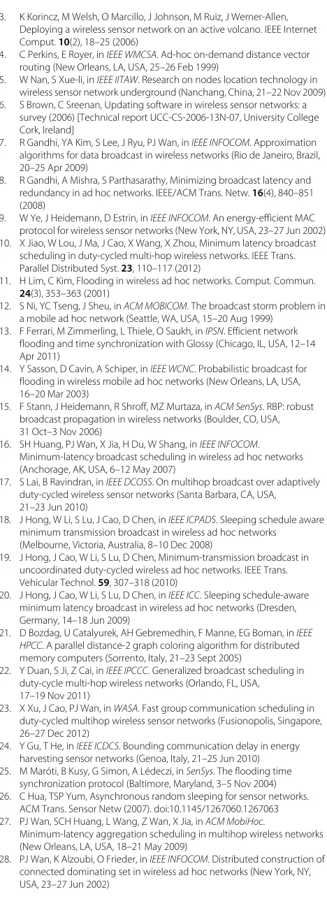
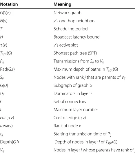
Figure 3The ranking and broadcast scheduling of shortest path treeTspt(G[U∪C])consisting of solid edges.The number inside each circle is a node’s rank, and the numbers in curly braces correspond to a node’s transmission times.

message tov7,v8, andv9. Accordingly, nodev6 ∈ U will get the message from nodev2which is adjacent to node v6andv7ofU. Nodev5will receive the message from a dominator inUsuch asv6.

ILBS then appliesfront-to-back orderingto color parent nodes inW1, i.e.,W1= {v3,v2}. As one of nodev3’s chil-dren, nodev7is also adjacent to nodev2, two colors will be needed to color them, i.e.,v3is colored 1, andv2is col-ored 2. That is,W1(1) = {v3}andW1(2)= {v2}. Nodev5 only gets the message fromv6 ∈ W2, sandv6is colored 1 as persmallest-degree-last ordering, i.e.,W2(1) = {v6}. The broadcast schedule can be presented asW(1)= {v3}, W(2)= {v2}, andW(3)= {v6}.

4.2 CFBS algorithm

Recall that the main idea of CFBS is to schedule transmis-sions in more than one layer to speed up the broadcast. This is achieved using three key steps: (1) computing a CDS ofG, (2) associating arankto nodes in the CDS, and (3) scheduling transmissions based on the constructed CDS and nodes’ ranks.

4.2.1 CDS construction

The NP-hard problem of computing a minimum CDS of Gis well studied, see [28,30,31], and references therein, and there are many approximation algorithms. However, for our problem, we not only require a small-size CDS but also one that has a small radius. To this end, we propose a new heuristic solution that achieves both objectives.

swill be the first node to be added intoU, and no nodes in layer 1 ofTspt(G)will be selected because they must be adjacent to nodes. The process then continues for layer 2 and so forth, whereby nodes at each layer which are not adjacent to those inUare selected greedily. From hereon, we will refer to nodes inUasdominators.

To ensure connectivity, the next step is to select con-nectornodes; recall thatG[U] is not connected as per the definition of MIS. LetUi be set of dominators in layeri, andCbe the set of selected connectors. The setCis pop-ulated layer by layer in a top-down manner. Specifically, a connector is chosen from nodes in an upper layerj, where j<i, that covers the most dominators inUithat have yet to be covered by other connectors. Upon completion, we thus haveG[U∪C], wherebyU∪Cis a CDS ofG.

Lemma 1.The resultant CDS satisfies the following

properties:

1. |U∪C| ≤2|U| −1≤2O(Rad(G,s)2)−1 2. Rad(G[U∪C],s)≤(T+1)Rad(G,s)−2T.

Proof. The first property is true because the connectors inCare required to cover at least one dominator located in a lower layer. Hence, the number of connectors|C|is bounded by |U| −1, which excludes the source nodes. The size of the CDS is thus bounded by 2|U| −1, which comprises|U|dominators and at most|U|−1 connectors. As proven in [27], the size of CDS for graphGis bounded byO(R2). This yields the inequality 2|U|−1≤2O(R2)−1. Recall thatR ≤ Rad(G,s), and thus we have|U∪C| ≤ 2|U| −1≤2O(Rad(G,s)2)−1.

For the second property, we first count the number of edges for a path from the source nodesto the maximum layer number, denoted asL, ofTspt(G). Observe that the dominators at layerLofTspt(G)will remain at the lowest layer ofTspt(G[U∪C]). The path from source nodesto a dominator at the lowest layer ofTspt(G[U∪C])consists of two kinds of edges: (1) the edge between two nodes in the same layer ofTspt(G)and (2) the edge between two nodes from different layers of Tspt(G). Therefore, in the worst case, there areL−2 edges of the first kind, i.e., from layer 2 toL−1 ofTspt(G), andLedges of the second kind.

Now, for the path cost, the edge cost between two nodes in the same layer isT because both nodes have the same active time slot, and thus, the total cost of theL−2 edges of the first kind mentioned earlier is thus(L−2)T. For the otherLedges of the second kind, their total cost will not exceed the radius ofG, i.e., Rad(G,s).

The total depth or cost to a dominator at the lowest layer ofTspt(G[U∪C])is thus Rad(G,s)+T(L−2). We know that the maximum layer numberLis no more than Rad(G,s), and thus, the total cost to the said dominator cannot exceed Rad(G,s)+T(Rad(G,s)−2) = (T +1)

Rad(G,s)−2T. As the said dominator lies at the lowest layer ofTspt(G[U∪C])and the depth of nodes in the low-est layer of the shortlow-est path tree is equal to the radius of G[U∪C], we thus have the required property.

4.2.2 Ranking process

The next step is to rank the nodes in the CDS. After which, in Section 4.2.3, CFBS will use the resulting ranks to construct a broadcast schedule, whereby nodes with the greatest rank will be scheduled to transmit first. A key property of ranking is that nodes with a higher rank is able to cover more nodes or relay a message further quicker, and thus reducing broadcast latency.

The ranking process starts by constructing the shortest path treeTspt(G[U∪C]). Then, CFBS assigns each node inG[U∪C] with a rank layer by layer in a bottom-up man-ner. Initially, for any nodev∈ U∪C, its rank is set to 0, i.e., rank(v) = 0. For each layeriofTspt(G[U∪C]), col-lect all nodes in layeriinto setMand repeat the following iteration untilMis empty. First, compute the maximum rankrof nodes inM. Then, find a nodeufrom an upper layer that covers the most nodes with rankrinM. If the rank of node u, i.e., rank(u), is more than r, rank(u) is unchanged; otherwise, it will be updated in the following way. Ifuis adjacent to only one node inMwith rankr, then rank(u)=r; otherwise, rank(u)=r+1. Mark node uas the parent of the chosen nodes with rankrinMand remove it fromM.

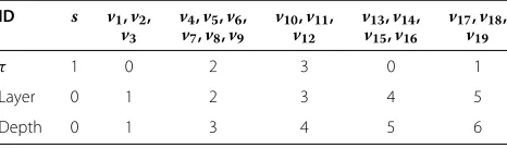
We now use Figure 3 to illustrate the ranking of Tspt(G[U∪C]). In our example,Tspt(G[U∪C])consists of 20 nodes, and the scheduling periodT is set to [0, 1, 2, 3]. Table 2 lists the active time slot, layer number, and depth information of all nodes inTspt(G[U∪C]).

Initially, all nodes in Figure 3 are assigned a rank of 0. Then, starting from the bottom layer, CFBS collects all nodes in layer 5 into setM, i.e.,M= {v17,v18,v19}. Next, nodev16 from layer 4 will be considered first because it covers the most number of nodes with rank 0 in layer 5, i.e.,v18andv19. Thus, nodev16’s rank will be updated to 1, i.e., rank(v16)=1 because it is adjacent to two nodes with rank 0, and its original rank is also 0. After that, nodesv18 andv19 are marked as the children of nodev16 and are removed from the set Mto yieldM = {v17}. Node v17 is only covered by node v11, and thus, nodev11 is set as

the parent ofv17, and its rank remains at 0. The other lay-ers are considered in a similar manner, and the maximum rank ofTspt(G[U∪C])is 2, i.e., rank(s)=2. parents, respectively, and all of them have the same rank, then neitherv2andu1noru2andv1are adjacent inG[U∪C];

3. The source node s has the maximum rank r, and r≤1+2O(log₂(Rad(G[U∪C] ,s))).

Proof.The first property is true due to how nodes obtain their rank. To prove the second property, assume that nodev2 is ranked beforeu2. Whenv2 is ranked, nodes v1andu1are in setMand have the same rankr. Hence, nodev1must be the only neighbor of nodev2with rank rin the setM. Otherwise, ifv2 has two neighbors with rank r in M, say node v1 and u1, the rank of node v2 must be more thanr. Therefore, the second property also holds true.

The first part of the third property is true because each node has a rank no more than its parent by the first prop-erty, and ranking is carried out in a bottom-up manner, and therefore, it follows that the source node s has the maximum rankr. Next, we show that rankris bounded byO(log₂(|U∪C|)). Denote byNithe number of nodes in layeriofTspt(G[U∪C])and byrithe maximum rank of nodes in layeri. LetLbe the maximum layer number of Tspt[G[U ∪C]]. First, observe that for any layer i, ri is no more thanrL +(L−i). As ranking is carried out from layerL, each additional layer thereafter increases a node’s rank by at most one, and thus for nodes in layeri, their rank increases by at most 1×(L−i), for a total of rL +(L−i). Furthermore, for any layeri−1, the num-ber of nodes with rankrL+(L−i)+1 does not exceed Ni/2 because in the worst case, every parent node in layer i−1 with rankrL+(L−i)+1 has two children in layer ithat has the maximum rankrL+(L−i), which means each parent node picks at most two children in layeriat a time, and the number of these said parent nodes isNi/2. By induction, we have for any layerithe number of nodes with rankrL+(L−i)does not exceedNL/2L−i, whereby

After computing the ranks of all nodes inG[U∪C], trans-missions are scheduled in two phases. In phase 1, CFBS schedules the transmission of nodes inG[U∪C], i.e., the CDS. In phase 2, it schedules transmissions from dom-inators inU ∪Cto all other nodes in G. The rationale for having two phases is that it is not necessary to send a message to non-CDS nodes early as they are not respon-sible for relaying the message further. On the other hand, by reducing the number of receiving nodes in phase 1, a transmitter will avoid a number of potential conflicts when sending a message to CDS nodes, thus reducing the broadcast latency.

In phase 1, transmissions are scheduled from the top to the bottom layer ofTspt(G[U∪C]). LetSij be the set of nodes with rankjthat are parent of nodes in layeri, and Vijbe the corresponding set of children in layeri. Apipe with rankj, denoted asPij, is defined as the transmissions from nodes inSijtoVij. Lettijbe the starting transmission time ofPij.

Initially, only nodesin layer 0 transmits a message at time slot 0. Then, for each layer i of Tspt(G[U ∪ C]), scheduling is carried out according to nodes’ rank, whereby the pipe with the highest rank is scheduled first. For instance, for layer 2 of Figure 3, CFBS first schedules pipeP21.

CFBS follows a greedy strategy to compute the mini-mumtij for each pipePij. The starting transmission time tijmust satisfy the following constraints:

(1) tijis larger than the reception time of nodes inSij, meaning a parent node inSijmust have received the message collision-free before it is allowed to transmit;

(2) to avoid collisions within the same layer,tijmust be larger than the reception time of nodes inVi(j+1)of pipePi(j+1)if it exists, that is, each pipePijstarts after pipePi(j+1)ends;

(3) to avoid collisions between different layers, we must have|tij−(Depth(G[U∪C],i)−1)|mod3T =0, where the time slot of(Depth(G[U∪C],i)−1)is the minimum or optimal receiving time of nodes in layeri ofTspt(G[U∪C]); this constraint thus ensures that the interval between transmissions is 3T, which guarantees that there are no inter-layer, interfering, and transmitting nodes.

reception time of parent nodes and other nodes that lie in the same layer, meaning, a parent node does not need to wait for all nodes in the upper layers to finish their transmission.

Next, CFBS schedules transmissions within pipe Pij. Denote byW₀ the set of nodes inVijwith rankj, andW0 is the set containing their respective parent, i.e.,W0⊆Sij. For each parent node vin W0, its transmission time is set totij. Then, CFBS applies ILBS to generate a broad-cast schedule (W(1),W(2),· · ·,W(l) ) for nodes in Sij andVij\W₀. For each 1 ≤ k ≤ l, ifW0 orW₀ is non-empty, all nodes inW(k)transmit at time slottij+3kT; otherwise, they transmit at time slot tij + 3(k − 1)T. Moreover, given that we have l ≤ 17, it follows that each pipe will take at most 51T time slots to finish transmission.

In phase 2, only a subset of dominators inU send the message to nodes in V \ (U ∪C). First, CFBS collects into a new subsetDiall the dominators that have a neigh-bor with active time slot Ti in set V \(U ∪C), where 0 ≤ Ti ≤ T −1. Then, it computes a partition ofDi into subsets Di(k)for 1 ≤ k ≤ cvia D2-coloring with smallest-degree-last ordering based on the rule that if two dominators share the same neighbor(s) with active time slot Ti in V \ (U ∪ C), they must not share the same color or be in the same subset. According to [10], we have c ≤ 12. Let Tp1 be the maximum transmission time of Phase 1, and thus in Phase 2, the transmission time of nodes in D(i)(k) is set to Tp1/T

T +kT + Ti, where 1 ≤ k ≤ 12 and 0 ≤ Ti ≤ T −1. Denote by Tp2 the maximum transmission time of phase 2. Hence, we get Tp2≤Tp1+12T.

Referring to Figure 3, after determining the ranks in Tspt(G[U ∪C]), the next step is to determine the trans-mission time of nodes inG[U∪C]. We start from pipe P12, which consists ofS12 = {s} andV12 = {v1,v2,v3}. Hence, the nodes in V12 will receive the message from nodesat time slot 0. Then, it considers nodes in layer 2. Among the parents in layer 2, i.e.,v1, v2, and v3, nodes v2andv3have the maximum rank 1. Hence, CFBS first schedules pipe P21, which comprisesS21 = {v2,v3}and V21= {v5,v6,v7,v8,v9}.

Both nodes inS21receive the message at time slot 0, and pipeP21 is the first one to be considered for layer 2, and thus the starting transmission timet21must be larger than 0. Moreover, it must satisfy|t21−(Depth(G[U∪C], 2)−1)| mod 3T =0. Recall thatT =4 and Depth(G[U∪C], 2)= 3; see Table 2. The minimum t21 is set to 2, i.e., t21 = min{t|t>0 and|t−2|mod 12=0} = 2. Set V21 does not contain nodes with rank 1, i.e., W0 = ∅, and thus the next step is to apply ILBS to schedule P21. As illus-trated in Section 4.1, sinceW(1)= {v3},W(2)= {v2}, and W(3) = {v6}in pipeP21, the transmission time ofv3,v2, andv6is set to 2, 14, and 26, respectively.

Then, pipeP20 is scheduled, wherebyS20 = {v1}and V20 = {v4}. Its starting transmission time t20 must be larger than nodev4’s reception time, i.e., 0, and larger than V21’s maximum reception time, i.e., 26. Hence, we have t20=min{t|t>0,t>26 and|t−2|mod 12=0} =38. The other layers are scheduled using a similar method, and the latency forTspt(G[U∪C])is 39. Moreover, from Figure 3, node v16 from layer 4 received the broadcast message from nodev12at time slot 4, which is smaller than the reception time of nodev1 from layer 1, i.e., 38. This demonstrates the advantage afforded by CFBS in allowing a node in a lower layer to receive earlier than a node in an upper layer.

4.3 Analysis

The next set of theorems assert the correctness of CFBS and establish its upper bound in terms of the broadcast latency and number of transmissions.

Theorem 1.CFBS provides a correct and collision-free

broadcast schedule.

Proof. Recall that CFBS performs transmissions in two phases. Thus, we only need to prove that all nodes in each phase are able to receive the broadcast message collision free. In phase 1, the broadcast is conducted pipe by pipe, and thus we need to prove that the transmissions in each pipe are collision free, and different pipes do not interfere with one another.

The theorem is true in phase 1 because CFBS schedules transmissions within each pipe using ILBS, which pro-duces a collision-free schedule. Next, we show that the transmissions between different pipes are also collision free. We prove this by considering two cases. In the first case, we consider pipes belonging to the same layer, sayi. Recall that for each layeri, pipePijstarts after pipePi(j+1)

finishes. Therefore, the pipes from the same layer will not interfere with each other.

in Tspt(G[U∪C]), that is, the reception time of nodes in layeri1andi2will not overlap with each other. Hence, in the second case, the pipes’ transmissions are also colli-sion free. Hence, CFBS yields a correct and collicolli-sion-free schedule in phase 1.

In phase 2, CFBS uses smallest-degree-last ordering D2-coloring method to divide dominators into different subsets; hence, as mentioned in [10], it is also collision free. Thus, the theorem is proven.

Lemma 3.For any pipe Pijof Tspt(G[U∪C]), its starting transmission time tijdoes not exceed Depth(G[U∪C],i)+ 54(r−j)T.

Proof.We prove this lemma by induction. For layer 0 ofTspt(G[U∪C]), it holds true because the transmission time of source nodesis zero. Assume this lemma is cor-rect for all layers before layeri. We now prove that it also holds true for layeri. Recall that the starting transmission time oftijis determined by two constraints: (1) maximum reception time ofSijand (2) maximum reception time of nodes inVi(j+1). Next, we analyze the correctness of this

lemma based on these two constraints.

First, we compute the maximum reception time of nodes in Sij. According to the definition of pipes, the nodes inSijare the parent of nodes in layeri, and hence they lie higher than layeri. Assume that nodev∈Sijlies in layeri1, wherei1<i. Note that the rank of nodev’s parent, denoted byj1, is no less thanv’s rankjby the first property of Lemma 2, i.e.,j1 ≥ j. Lemma 3 is correct for layeri1, and therefore, the starting transmission timeti₁j1 of pipe Pi₁j1 is no more than Depth(G[U∪C],i1)+54T(r−j1), i.e.,ti1j1 ≤Depth(G[U∪C],i1)+54T(r−j1); recall that ris the maximum rank, i.e.,rank(s) =r. Each pipe takes at most 51T to finish its transmission, and hence, when j<j1, nodevwill receive the message after pipePi1j1 fin-ishes at time Depth(G[U∪C],i1)+54T(r−j1)+51T ≤ Depth(G[U ∪C],i1)+ 54T(r− j). On the other hand, whenj=j1, nodevwill receive the message from its par-ent at the starting transmission timeti1j1 =Depth(G[U∪ C],i1)+54T(r−j). Hence, for nodev, its maximum recep-tion time is no more than Depth(G[U∪C],i1)+54T(r−j). Furthermore, since Depth(G[U∪C],i) > Depth(G[U∪ C],i1), node v’s maximum reception time is less than Depth(G[U∪C],i)+54T(r−j).

Second, we analyze the maximum reception time of nodes inVi(j+1). Assume that the maximum rank of nodes

in layer iis ri, i.e., ri ≥ j. For layeri, the transmission starts from the pipe with greatest rank, and hence, for pipe Piri, its starting transmission timetiri is only determined by the maximum reception time of nodes inSiribecause nodes with rank ofri+1 for layerido not exist. Recall that the maximum reception time of nodes inSiri is less than Depth(G[U∪C],i)+54T(r−ri), and thus in the worst case,

for pipePiri,tiriis set to Depth(G[U∪C],i)+54T(r−ri). Since each pipe takes up at most 51T time slots, and the reception time of nodes in layeriis separated by 3T, we have ti(j+1) − tiri ≤ (ri − (j + 1))54T. Therefore, for nodes inVi(j+1), their maximum reception time is no more

than Depth(G[U∪C],i)+54T(r−(j+1))+51T, i.e., Depth(G[U∪C],i)+54T(r−ri)+54T(ri−(j+1))+51T. By considering both reception time of nodes in Sij andVi(j+1), this means in the worst case,tij is equal to Depth(G[U∪C],i)+54T(r−j), which proves the required bound oftij≤Depth(G[U∪C],i)+54T(r−j). Thus, this lemma is also true for layeri. Note that, 54Tcorresponds to 51Twhich is the number of time slots for each pipe to finish its transmission and 3Twhich is the interval used to separate the stating transmission time between adjacent pipes.

Corollary 1.Algorithm CFBS produces a broadcast

schedule with latency(T+1)H+TO(log₂H), where H is Rad(G[U∪C],s).

Proof.By Lemma 3, it is clear that the latency in phase 1 is at most Depth(G[U ∪C] ,L) +54rT, where the latency in phase 1 is therefore bounded by (T+1)H+108TO(log₂H)+52T. That is, in phase 1, the broadcast latency is bounded by(T+1)H+TO(log₂H), whereby the omitted constant before TO(log₂H) is 108.

The second phase of CFBS takes at most 12Ttime slots, and hence, the broadcast latency of CFBS is bounded by (T+1)H+TO(log₂H)+12T =(T+1)H+TO(log₂H).

Theorem 2.CFBS is a4(T +2)-approximate solution

in terms of number of transmissions.

of U does not exceed 4opt+1 [28], whereoptdenotes the minimum number of transmissions. CFBS is thus a (T+2)(4opt+1)−1 solution.

4.4 Remarks on always-on wireless networks

CFBS is also applicable for always-on wireless networks, whereT is set to one. Specifically, it starts by construct-ing a breadth-first search tree (BFS) rooted at the source nodes. Here, the BFS tree is a special case ofTspt, where the cost of each edge in a given network is fixed to one. Then, CFBS builds the dominator set U and connector set C based on the BFS tree in the same way as illus-trated in Section 4.2.1, where dominators in U together with connectors in C form a CDS. The next step is to build a new BFS tree rooted at the source based on graph G[U ∪C], then followed by a ranking of the nodes in this new BFS tree layer by layer in a bottom-up manner via the same method in Section 4.2.2. Note, for a given always-on wireless network G, its radius with respect to the source node s, i.e., Rad(G,s), is equal toR. sThis is because the cost of each edge inGis one whenT = 1. Also note that Lemmas 1 and 2 still hold true for always-on wireless networks. In particular, as stated in Lemma 1, Rad(G[U∪C] ,s)≤2R−2. As shown by Lemma 2, each nodevinG[U∪C] has a rank no more than its parent and rank(v)≤1+2O(log₂(2R−2).

In the third step, the broadcast scheduling process for always-on wireless networks also consists of two phases: (1) broadcast data to all nodes in the CDS and (2) broad-cast data from dominators to remaining nodes. In the first phase, for each pipe Pij, its staring transmission time tij will be first calculated according to the same greedy method described in Section 4.2.3. Then, the par-ent whose corresponding child has a rank ofjin pipePij is scheduled to transmit attij. For the other nodes inPij, CFBS applies the ILBS algorithm in Section 4.1 to generate a broadcast schedule. Note that during calculation, sthe scheduling periodT is always set to one. In the second phase, CFBS partitions the dominators into different sub-sets using D2-coloring with smallest-degree-last ordering, where the dominators in the same subset have the same color. Then, these dominators transmit based on their color.

Similar to Corollary 1, CFBS produces a 2R+O(log₂R) -approximate solution in terms of the broadcast latency. Note that for always-on wireless networks, the optimal broadcast latency is equal toR, that is,H= R. According to Theorem 2, we can see that CFBS is a 12-approximation solution with respect to the number of transmissions. Compared with the best multiplicative approximation algorithm to date for always-on networks, i.e., [7] that gives a broadcast latency bound of 12R, our addictive approximation algorithm has a lower latency bound of 2R+O(log₂R).

Furthermore, in CFBS, the omitted constant in

O(log₂R) is less than 108. Compared with the addictive approximation algorithm in [16], which has a latency bound ofR+O(log₂R), but with an omitted constant in

O(log₂R)that exceeds 150, our broadcast bound will be smaller whenRbecomes larger.

5 Evaluation

In this section, we outline the research methodology used to evaluate the performance of CFBS. We compare CFBS against OTAB [10], which is known to have the lowest constant approximation ratio to date. In our experiments, we measure each algorithm against two metrics:

• Broadcast latency: this is defined as the total time required by all nodes to receive a broadcast message;

• Transmission ratio: this is the ratio between the number of transmissions and the number of nodes.

That is, the transmission ratio represents the average number of messages retransmitted by each node in the network. It is worth pointing out that the main goal of our simulation is to compare the theoretical and experimen-tal broadcast latency and transmission ratio performance of our algorithm. In particular, the latency is mainly deter-mined by the nodes’ interwake-up times, which are a few orders of magnitude higher than the length of a slot. Moreover, in Section 3.1, it is assumed that a message can be successfully delivered from a sender to a receiver within a time slot. In reality, as shown in [24], the max-imum size of a typical TinyOS packet is 47 bytes, a time slot is usually set to 20 ms, and thus, a MicaZ node can attempt at least 13 transmissions in one time slot. In other words, although low-power wireless links are gen-erally unreliable, we can still ensure that a message can be successfully transmitted within a time slot through multi-ple transmissions [24]. Therefore, in our simulations, we only consider the packet loss caused by collisions, and assume that unreliable links can be solved within a time slot through multiple transmissions. It is for this reason we do not employ a packet level simulator and any specific MAC protocols.

Figure 4Broadcast latency under different network sizes.

remain unchanged. Each experiment is conducted on 20 randomly generated topologies. Moreover, for each topol-ogy, we carry out the experiment for 10 runs, and in each run, an arbitrary node is selected as the source node. Hence, each result is the average of 200 simulation runs.

5.1 Impact of network size

Figure 4 presents the average broadcast latencies of CFBS and OTAB when we vary the network size, which is denoted by the square length l. In this experiment, the number of nodes, transmission radius, and duty cycle are set to 400, 30 m, and 0.05, respectively. In Figure 4, we observe that the broadcast latency of both algorithms grows proportionally to the square of lengthl. The reason is as follows. The broadcast latency of CFBS and OTAB is mainly influenced by the number of layers in the SPT. For a fixed number of nodes and transmission radius, the network becomes sparse when we increase the network size. As a result, the network has fewer links and connec-tivity, and thus SPT has more layers. Furthermore, CFBS performs much better than OTAB, i.e., when the square length is set to 350 m, the broadcast latency of CFBS is

Figure 5Transmission ratio under different network sizes.

Figure 6Broadcast latency under different number of nodes.

only 1₈ that of OTAB. This is because instead of schedul-ing transmissions layer by layer as in OTAB, CFBS is able to schedule nodes’ transmission in more than one layer, which helps reduce the broadcast latency.

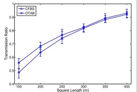
Figure 5 plots the transmission ratio versus the net-work size. We find that the transmission ratio for CFBS and OTAB grows with increasing network size. This is because the average degree decreases when we increase the network size; thereby, a node will inform fewer nodes after each transmission. This means a node requires more transmissions to cover its neighbors. Moreover, CFBS per-forms better than OTAB in terms of the transmission ratio. This is because CFBS selects transmitting nodes from a small CDS.

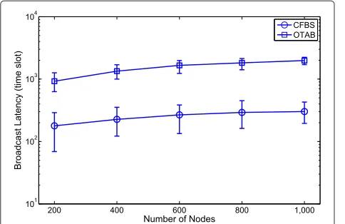
5.2 Impact of node numbers

In Figure 6, we present the average broadcast latencies of CFBS and OTAB when we change the number of nodes. In this experiment, the square length, transmis-sion radius, and duty cycle are fixed at 200 m, 30 m, and 0.05, respectively. As shown in Figure 6, we find that the broadcast latency of both algorithms grows as the

Figure 8Broadcast latency under different transmission radii.

number of nodes increases. This is because the network becomes denser when the number of nodes increases in a fixed network area. As a result, there are more links and richer connectivity, and thus, the SPT rooted at the source produces fewer layers. That is, less time will be required to inform all nodes. Furthermore, CFBS per-forms much better than OTAB, i.e., when the number of nodes is set to 1,000, the broadcast latency of CFBS is only ₂₀3 that of OTAB, for the same reason as listed in Section 5.1.

Figure 7 shows the transmission ratio versus the number of nodes. We see that the transmission ratio for both algo-rithms decreases with increasing number of nodes. This is because the average degree grows with increasing num-ber of nodes; thereby, a node can inform more neighbors via one transmission. This means a node requires fewer transmissions to cover its neighbors. Moreover, CFBS still performs better than OTAB in terms of transmission ratio.

Figure 9Transmission ratio under different transmission radii.

Figure 10Broadcast latency under different duty cycles.

5.3 Impact of transmission radius

In Figure 8, we plot the broadcast latencies of CFBS and OTAB under different transmission radii. In this experi-ment, we set the square length, number of nodes. and the duty cycle to 200 m, 400, and 0.05, respectively. We see that the broadcast latency of both algorithms decreases with increasing transmission radius. This is because the nodes with a larger transmission radius will have higher connectivity with other nodes, which helps reduce the number of layers in the SPT. Notably, CFBS performs much better than OTAB in terms of the broadcast latency under different transmission radii, i.e., the latency of CFBS is within 17% of the latency achieved by OTAB.

Figure 9 shows that the transmission ratio of CFBS and OTAB decreases as the transmission radius grows. This is due to nodes with larger transmission radius being able to inform more nodes in one transmission, and thus, fewer transmissions will be needed to inform its neighbors. Fur-thermore, CFBS has a better performance in terms of the transmission ratio as compared to OTAB.

5.4 Impact of duty cycle

Figure 10 is a plot of the broadcast latency versus duty cycle. We fix the square length to 200 m, the number of nodes to 400, and the transmission radius to 20 m. From Figure 10, we find that the broadcast latency of CFBS and OTAB increases with declining duty cycle. The reason is due to the scheduling periodT containing more time slots as the duty cycle decreases; a node will thus need to wait longer before forwarding a message to its neigh-bors. In addition, CFBS performs much better than OTAB in terms of the broadcast latency, i.e., CFBS’s broadcast latency is around 15% that of OTAB when the duty cycle is set as 0.02.

Figure 11 shows that the transmission ratio for both algorithms increases with decreasing duty cycle. When the duty cycle decreases, the scheduling periodTwill con-tain more time slots, and a node needs to transmit more times to inform its neighbors because they have a higher probability of choosing different active time slots from a largerT. Moreover, CFBS outputs a smaller transmission ratio than OTAB.

6 Conclusion

This paper has formally outlined the MLBSDC prob-lem and presented a novel algorithm called CFBS with a broadcast latency of at most(T +1)H+TO(log₂H). In addition, we proved that CFBS provides a correct and collision-free broadcast scheduling and achieves a low latency and overhead in terms of the number of trans-missions. Our simulation results indicate that CFBS has a better performance, in terms of the broadcast latency and transmission ratio, than OTAB under different network configurations.

As a future work, we are currently looking into imple-menting CFBS in distributed manner. The use of our method under the physical interference model is another possible future work. Under this model, we need to con-sider both collisions and total interference from nearby transmitters.

Competing interests

The authors declare that they have no competing interests.

Acknowledgements

This project is supported by the CSC-UoW joint scholarship program.

Received: 21 January 2013 Accepted: 11 October 2013 Published: 23 October 2013

References

1. A Baggio, inACM REALWSN. Wireless sensor networks in precision agriculture (Stokholm, Sweden, 20–21 Jun 2005)

2. W Hu, VN Tran, N Bulusu, C Chou, S Jha, A Taylor, inACM/IEEE IPSN. The design and evaluation of a hybrid sensor network for cane toad monitoring (Los Angeles, CA, USA, 15 Apr 2005)

3. K Korincz, M Welsh, O Marcillo, J Johnson, M Ruiz, J Werner-Allen, Deploying a wireless sensor network on an active volcano. IEEE Internet Comput.10(2), 18–25 (2006)

4. C Perkins, E Royer, inIEEE WMCSA. Ad-hoc on-demand distance vector routing (New Orleans, LA, USA, 25–26 Feb 1999)

5. W Nan, S Xue-li, inIEEE IITAW. Research on nodes location technology in wireless sensor network underground (Nanchang, China, 21–22 Nov 2009) 6. S Brown, C Sreenan, Updating software in wireless sensor networks: a

survey (2006) [Technical report UCC-CS-2006-13N-07, University College Cork, Ireland]

7. R Gandhi, YA Kim, S Lee, J Ryu, PJ Wan, inIEEE INFOCOM. Approximation algorithms for data broadcast in wireless networks (Rio de Janeiro, Brazil, 20–25 Apr 2009)

8. R Gandhi, A Mishra, S Parthasarathy, Minimizing broadcast latency and redundancy in ad hoc networks. IEEE/ACM Trans. Netw.16(4), 840–851 (2008)

9. W Ye, J Heidemann, D Estrin, inIEEE INFOCOM. An energy-efficient MAC protocol for wireless sensor networks (New York, NY, USA, 23–27 Jun 2002) 10. X Jiao, W Lou, J Ma, J Cao, X Wang, X Zhou, Minimum latency broadcast

scheduling in duty-cycled multi-hop wireless networks. IEEE Trans. Parallel Distributed Syst.23, 110–117 (2012)

11. H Lim, C Kim, Flooding in wireless ad hoc networks. Comput. Commun. 24(3), 353–363 (2001)

12. S Ni, YC Tseng, J Sheu, inACM MOBICOM. The broadcast storm problem in a mobile ad hoc network (Seattle, WA, USA, 15–20 Aug 1999)

13. F Ferrari, M Zimmerling, L Thiele, O Saukh, inIPSN. Efficient network flooding and time synchronization with Glossy (Chicago, IL, USA, 12–14 Apr 2011)

14. Y Sasson, D Cavin, A Schiper, inIEEE WCNC. Probabilistic broadcast for flooding in wireless mobile ad hoc networks (New Orleans, LA, USA, 16–20 Mar 2003)

15. F Stann, J Heidemann, R Shroff, MZ Murtaza, inACM SenSys. RBP: robust broadcast propagation in wireless networks (Boulder, CO, USA, 31 Oct–3 Nov 2006)

16. SH Huang, PJ Wan, X Jia, H Du, W Shang, inIEEE INFOCOM. Minimum-latency broadcast scheduling in wireless ad hoc networks (Anchorage, AK, USA, 6–12 May 2007)

17. S Lai, B Ravindran, inIEEE DCOSS. On multihop broadcast over adaptively duty-cycled wireless sensor networks (Santa Barbara, CA, USA, 21–23 Jun 2010)

18. J Hong, W Li, S Lu, J Cao, D Chen, inIEEE ICPADS. Sleeping schedule aware minimum transmission broadcast in wireless ad hoc networks

(Melbourne, Victoria, Australia, 8–10 Dec 2008)

19. J Hong, J Cao, W Li, S Lu, D Chen, Minimum-transmission broadcast in uncoordinated duty-cycled wireless ad hoc networks. IEEE Trans. Vehicular Technol.59, 307–318 (2010)

20. J Hong, J Cao, W Li, S Lu, D Chen, inIEEE ICC. Sleeping schedule-aware minimum latency broadcast in wireless ad hoc networks (Dresden, Germany, 14–18 Jun 2009)

21. D Bozdag, U Catalyurek, AH Gebremedhin, F Manne, EG Boman, inIEEE HPCC. A parallel distance-2 graph coloring algorithm for distributed memory computers (Sorrento, Italy, 21–23 Sept 2005)

22. Y Duan, S Ji, Z Cai, inIEEE IPCCC. Generalized broadcast scheduling in duty-cycle multi-hop wireless networks (Orlando, FL, USA, 17–19 Nov 2011)

23. X Xu, J Cao, PJ Wan, inWASA. Fast group communication scheduling in duty-cycled multihop wireless sensor networks (Fusionopolis, Singapore, 26–27 Dec 2012)

24. Y Gu, T He, inIEEE ICDCS. Bounding communication delay in energy harvesting sensor networks (Genoa, Italy, 21–25 Jun 2010) 25. M Maróti, B Kusy, G Simon, A Lédeczi, inSenSys. The flooding time

synchronization protocol (Baltimore, Maryland, 3–5 Nov 2004) 26. C Hua, TSP Yum, Asynchronous random sleeping for sensor networks.

ACM Trans. Sensor Netw (2007). doi:10.1145/1267060.1267063 27. PJ Wan, SCH Huang, L Wang, Z Wan, X Jia, inACM MobiHoc.

Minimum-latency aggregation scheduling in multihop wireless networks (New Orleans, LA, USA, 18–21 May 2009)

29. DW Matula, LL Beck, Smallest-last ordering and clustering and graph coloring algorithms. J. ACM.30(3), 417–427 (1983)

30. S Guha, S Khuller, Approximation algorithms for connected dominating sets. Algorithmica.20(4), 374–387 (1998)

31. J Wu, M Gao, I Stojmenovic, inICPP. On calculating power-aware connected dominating sets for efficient routing in ad hoc wireless networks (Valencia, Spain, 3–7 Sept 2001)

doi:10.1186/1687-1499-2013-248

Cite this article as:Zhao and Chin:Approximation algorithm for data broadcasting in duty cycled multi-hop wireless networks.EURASIP Journal on Wireless Communications and Networking20132013:248.

Submit your manuscript to a

journal and benefi t from:

7 Convenient online submission 7 Rigorous peer review

7 Immediate publication on acceptance 7 Open access: articles freely available online 7 High visibility within the fi eld

7 Retaining the copyright to your article