R E S E A R C H
Open Access
The Euler scheme for stochastic differential
equations with discontinuous drift
coefficient: a numerical study of the
convergence rate
S. Göttlich
1*, K. Lux
1and A. Neuenkirch
1*Correspondence:
1Department of Mathematics,
University of Mannheim, Mannheim, Germany
Abstract
The Euler scheme is one of the standard schemes to obtain numerical approximations of solutions of stochastic differential equations (SDEs). Its
convergence properties are well known in the case of globally Lipschitz continuous coefficients. However, in many situations, relevant systems do not show a smooth behavior, which results in SDE models with discontinuous drift coefficient. In this work, we analyze the long time properties of the Euler scheme applied to SDEs with a piecewise constant drift and a constant diffusion coefficient and carry out intensive numerical tests for its convergence properties. We emphasize numerical convergence rates and analyze how they depend on the properties of the drift coefficient and the initial value. We also give theoretical interpretations of some of the arising
phenomena. For application purposes, we study a rank-based stock market model describing the evolution of the capital distribution within the market and provide theoretical as well as numerical results on the long time ranking behavior.
MSC: 60H10; 65C20
Keywords: Discontinuous drift; Numerical schemes; Convergence rates; Experimental study
1 Introduction
In recent years, many applications related to stochastic differential equations (SDEs) with discontinuous drift coefficient have emerged. These types of equations typically arise in mathematical finance and insurance [2,9,15,16], engineering applications [22,36], eco-nomy [26,38], or stochastic control problems [3,21,38,41].
The existence and uniqueness of solutions of SDEs in the standard case, i.e., the case of sufficiently smooth coefficients, are well understood [17], and the corresponding numeri-cal analysis is well developed (see, e.g., [19]) providing a variety of different numerinumeri-cal ap-proximation schemes. A recent numerical comparison of two of them, the Euler scheme and the Milstein scheme, in the case of nonlinear drift and diffusion coefficients can be found in [5].
However, the standard theory on SDEs does not apply anymore in case of a disconti-nuous drift coefficient, e.g., a piecewise constant drift coefficient, and a special theory is
needed to address the question of existence and uniqueness of solutions of such SDEs [18,42,44]. The same is true for the numerical analysis: The convergence behavior of approximation schemes needs to be reconsidered and “research on numerical methods for SDEs with irregular coefficients is highly active” [25, p. 2]. In the case of a sufficiently smooth drift and a constant diffusion coefficient, the exact strong rate of convergence is 1 for the Euler scheme, see [6,19]. At the time when the main part of the research presented here was undertaken, no comparable result was known in the case of a discontinuous, e.g., piecewise constant, drift coefficient. After many discussions and investigations, also inspired by a previous version of this manuscript, refined results are now about to be es-tablished, see Sect.2.1.
In this work, we focus on numerical approximations of SDEs in the presence of a piece-wise constant drift and a constant diffusion coefficient. We provide theoretical considera-tions on the long time behavior of approximated SDE soluconsidera-tions based on the results from the theory of ergodic Markov chains. Moreover, we provide further insight into the nu-merical behavior of approximation schemes, in particular the Euler scheme, by analyzing the numerical convergence rates based on a reference solution. The numerical speed of convergence heavily depends on the initial value and properties of the drift coefficient, e.g., drift direction or jump height. Our tests reveal that for a special class of drift coefficients the numerical convergence rates are higher and independent of initial conditions due to the ergodicity of the Euler scheme and the underlying SDE. In addition to focusing on the numerical convergence rates, we also use the Euler scheme to verify qualitative properties such as the long time behavior of a rank-based stock market model [4], a prominent model in finance to describe the evolution of the capital distribution within the market.
The remainder of this manuscript is as follows: In Sect.2, we introduce some theoretical and numerical basics and establish the ergodicity of the Euler approximations in the case of an appropriate, piecewise constant drift coefficient. In Sect.3, we discuss numerical convergence properties and further findings of several numerical tests. We conclude this work in Sect.4with the application from mathematical finance mentioned above, where SDEs with a discontinuity in the drift coefficient naturally arise.
2 Problem description
In this section, we introduce our basic setting, i.e., the type of SDE we are interested in and some basic terms for the numerical tests. Besides the Euler scheme and its long time properties in our setting, we also briefly discuss the applicability and performance of some other numerical schemes.
2.1 The equation
In this manuscript, we consider time-homogeneous SDEs with piecewise constant drift coefficient and additive noise:
dXt=
s
j=1
αj·1Bj(Xt)dt+σdWt, t≥0, X0=ξ. (1)
Here, we haves∈N,αj,σ,ξ∈Rand disjoint (possibly infinitely many) intervalsBj⊂R
for all 1≤j≤s, and (Wt)t∈[0,T]is a one-dimensional Brownian motion.
which the corresponding SDE has a unique strong solution, are derived. As emphasized therein, those conditions are in particular fulfilled for a bounded drift coefficient and a constant diffusion coefficient. Thus, the existence and uniqueness of a strong solution for SDEs of type (1) is ensured.
For the numerical analysis of SDEs with discontinuous drift and/or diffusion coefficient, the situation is more involved. In this manuscript, we focus on the strong convergence rate of the Euler scheme, which, for a general SDE
dXt=f(Xt)dt+g(Xt)dWt, t∈[0,T], X0=ξ,
wheref andgare such that a unique strong solution exists, is given by
xexpk+1E=xexpk E+fxexpk E+gxexpk E(W(k+1)–Wk), k= 0, . . . ,n– 1,
xexp0 E=ξ.
(2)
The underlying time discretization of the time interval [0,T] is 0 =t0<t1<· · ·<tn=T with corresponding step size:=Tn, wheren+ 1 is the number of grid points.
While its behavior is well known for SDEs with Lipschitz continuous coefficientsf and
g, much less has been known in more general cases, even for SDEs with additive noise and a piecewise constant drift coefficient. The first contribution in this area is—up to the best of our knowledge—the work [12], where almost sure convergence of the Euler scheme has been established in the case of a one-sided Lipschitz drift coefficient, a locally Lipschitz diffusion coefficient, and the existence of a Lyapunov function for the SDE. The results of [13] give strong convergence of the Euler scheme for SDEs with additive noise in the case of a discontinuous but monotone drift coefficient, while [40] establishes the almost sure and strong convergence of the Euler scheme for SDEs with additive noise and drift of the formf(x) = –sign(x). Recent contributions with respect to strong approximations of SDEs with discontinuous drift coefficient are a series of articles by Ngo and Taguchi [33– 35] and Leobacher and Szölgyenyi [23–25], respectively. Very recently Müller-Gronbach and Yaroslavtseva [29] established strong order 1/2 for (2) in the case of a scalar equation with piecewise Lipschitz drift and non-additive noise, and Neuenkirch et al. obtained the same convergence order for an adaptive Euler scheme in the multi-dimensional case, see [31]. The weak approximation of SDEs with discontinuous coefficients has been studied in [20], where an Euler-type scheme based on an SDE with mollified drift coefficient is analyzed.
In the case of SDE (1), the latest result on the strong convergence rate of the Euler scheme
xexpk+1E=xexpk E+
s
j=1
αj·1Bj
xexpk E+σ(W(k+1)–Wk), k= 0, . . . ,n– 1,
xexp0 E=ξ,
(3)
for the approximation ofXT, i.e., the solution at timeT, is anL2-convergence order 3/4 –ε in [30] for arbitrarily smallε> 0.
So to summarize: The Euler scheme for our non-standard setting of SDE (1) has at least
L2-convergence order 3/4 –ε. However, observing this convergence order numerically will be a different story (see Sect.3). For our theoretical and numerical considerations, we restrict ourselves to the case ofs= 2 in equation (1). This entails that we focus on one point of discontinuity in the drift coefficient to better work out the arising effects.
2.2 Error measurement
As already mentioned, we are interested in empirically measuring the strong convergence rate of the Euler scheme. The standard procedure for this is as follows: The root mean squared error (RMSE) at timeTfor Euler scheme (1) with step size=T/nis given by
e(n) :=EXT–xexpn E
21/2
. (4)
Since an explicit form ofXT is unknown in general, one needs to replaceXT in our
si-mulation studies by a numerical reference solutionXnum
T , which is computed by the Euler
scheme for an extremely small step size=T/Nwith a very large number ofN+ 1 grid points such that this approximation can be considered close enough to the true solution. Moreover, also the expectationE|Xnum
T –x expE
n |2is not known explicitly, so we will
approx-imate this expectation by the empirical RMSE
eemp(n) =
with a large numberMof Monte Carlo repetitions, i.e., (Xnum
T –x
n have the same random input. Note that Nhas to be chosen sufficiently large to generate the numerical reference solution and to avoid oscillations ineemp(n), which might occur ifN andnare close. If this is the case, solutions might either be almost identical (differences close to machine accuracy) or obey a difference as high as the full jump height (not captured drift changes). Those different scales might lead to oscillations in the error measurement. The number of repetitionsM
should also be large enough to have a good approximation of the expectation, i.e., a small Monte Carlo error.
An alternative error measurement that is often used is based on error increments and reads as follows:
In Sect.3, the numerical investigations are primarily based on error measure (5) and are supplemented by results obtained for error measure (6).
2.3 Other schemes
2.3.1 The implicit Euler scheme
Implicit schemes have good stability properties, thus they are a natural choice to consider. For an SDE with additive noise, where the drift coefficient is sufficiently smooth, the im-plicit Euler scheme has strong convergence order 1 (see, e.g., [1] and [32]).
However, for SDEs of type (1) already the implicit Euler scheme is not well defined. To see this, consider the SDE
requires to solve, for fixed but arbitraryz∈R, the equation
y–α1·1(–∞,0)(y) +α2·1[0,∞)(y)
=z,
with respect toy∈R. This equation does not possess a solution ifz∈(–α1, –α2), and hence an implicit Euler scheme is not well defined in this setting.
2.3.2 The Heun scheme
The Heun scheme is another scheme with strong order one for SDEs with additive noise under appropriate smoothness conditions on the drift coefficient. Adapted from [19, p. 373] for SDEs of type (1), it is defined by
For a closer look at the behavior of this scheme at a discontinuity, assume that the drift coefficient is given bya(x) =±sign(x). An increment of the Heun scheme withxHeun and an Euler step coincide. However, if a drift change occurs in the Euler step, the Heun step reads as
xHeunk+1 =x+σ(W(k+1)–Wk),
2.3.3 A Wagner–Platen type scheme
A strong order 1.5-scheme for SDEs with smooth drift coefficient and additive noise is given by a Wagner–Platen type scheme (see, e.g., [19, p. 383]), which reads in our setting as follows:
have the same sign or not. If this condition is fulfilled, i.e., ifxis sufficiently far away from the discontinuity, then a Wagner–Platen step and an Euler step coincide. If the latter con-dition is not satisfied, then we have the dynamics
xPlak+1=x+1
So, also here, the diffusive dynamic dominates the scheme when taking values close to the discontinuity.
2.4 Ergodicity and stability of the Euler scheme
We will now address the long time properties of the Euler scheme based on the results from the theory of ergodic Markov chains. Within the SDEs of type (1) withs= 2, we distinguish the equations with respect to the direction in which the drift coefficient is pointing.
Definition 1 We will call a drift coefficienta:R→Rinward pointingif there existsx∗∈ Rsuch that
a(x) > 0, x<x∗, a(x) < 0, x>x∗,
andoutward pointingif there existsx∗∈Rsuch that
In this subsection, we consider the special case of
i.e., an inward pointing drift coefficient towards the discontinuity zero. Clearly, we have
lim
s→0E(Xt+s|Xt=x) =x+α1·1(–∞,0)(x) +α2·1[0,∞)(x), t≥0,x= 0, (7)
i.e., on average, the solution is moving inwards. Moreover, following, e.g., Chap. 6 in [10], this SDE admits a unique invariant distribution with Lebesgue density
ϕ∞(x) =c·e2α2x·1[0,∞)(x) +c·e2α1x·1(–∞,0)(x), x∈R,
and the law of large numbers
lim It will turn out that the explicit Euler scheme
xkexp+1E,ξ=xexpk E,ξ+axkexpE,ξ+W(k+1)–Wk, k= 0, 1, . . . , x
expE,ξ
0 =ξ, (10)
with
a(x) =α1·1(–∞,0)(x) +α2·1[0,∞)(x), x∈R,
will recover these properties. (Here we also indicate the dependence on the initial value
ξ in our notation.) Euler scheme (10) corresponds to a time homogenous Markov chain with transition kernel
and satisfies the discrete counterpart to (7), i.e.,
Now, we will prove the existence of a unique stationary distribution for the Euler scheme. In particular, due to the discontinuity at zero, the following Proposition2is not covered by the standard references as, e.g., [27] and [37] for Euler-type discretizations of ergodic SDEs. Note that the long time properties of (10) have also been heuristically studied in [39]. Here, using the theory of Markov chains, we obtain the following geometric ergodi-city result for the Euler scheme.
Proposition 2 Letα1> 0 >α2and> 0be fixed.Then Euler scheme(10)admits a unique
stationary distributionμ,which is independent of the initial valueξ.Moreover,there exist
β∈(0, 1)and constantsM(ξ),ξ∈R,such that
sup A∈B(R)
P
xexpk E,ξ∈A–μ(A)≤M(ξ)·βk, k≥1.
Proof We start by verifying thatV(x) =eτ|x|,x∈R, is an appropriate Lyapunov function for the above Markov chain ifτ> 0 is sufficiently small. This is a direct consequence of the well-known form of the moment generating function for the folded normal distribution, i.e.,
Eeτ|μ+νW1|=eν 2τ2
2 +μτ1 –Φ(–μ/ν–ντ)+eν
2τ2
2 –μτ1 –Φ(μ/ν–ντ), τ∈R, (12)
whereΦis the distribution function of the standard normal distribution andμ∈R,ν> 0. Using (12) withμ=x+a(x)andν2=, we obtain
EVxexpk+1E,ξ|xexpk E,ξ =x≤eτ(τ2+|α2|)+eτ(2τ–|α2|)eτx, x≥0, EVxexpk+1E,ξ|xexpk E,ξ =x≤eτ(τ2+|α1|)+eτ(2τ–|α1|)e–τx, x< 0.
So, we have
EVxexpk+1E,ξ|xkexpE,ξ =x≤eτ(τ2+max{|α1|,|α2|})+eτ(τ2–min{|α1|,|α2|})eτ|x|, x∈R,
and choosingτ< 2min{|α1|,|α2|}gives the desired Lyapunov property
EVxexpk+1E,ξ|xkexpE,ξ =x≤C+γV(x), x∈R,
withC> 0,γ ∈(0, 1). Since the transition kernel is Gaussian, an application of the quan-titative Harris theorem (see, e.g., Chap. 15 in [28], or Theorem 3.15 (and the following example) in [7]) yields the geometric ergodicity result.
ChoosingA= (–∞,y], we obtain in particular the counterpart to (8), i.e.,
lim k→∞P
xexpk E,ξ ≤y=μ
(–∞,y], y∈R. (13)
Moreover, an ergodic theorem as, e.g., Corollary 2.5 in [7] yields also the discrete coun-terpart to the law of large numbers (9): We have
lim L→∞
1
L L
k=1
hxexpk E,ξ=
∞
–∞h(x)
μ(dx) a.s., (14)
for all measurableh:R→Rsuch that–∞∞ |h(x)|μ(dx) <∞.
Finally, note that SDEs with outward pointing drift coefficients do not admit a stationary solution. For the SDE
dXt=α1·1(–∞,0)(Xt) +α2·1[0,∞)(Xt)
dt+dWt, t≥0, X0=ξ,
withα1< 0 <α2, straightforward calculations using It¯o’s lemma yield
E|Xt|2≥ξ2+t, t≥0,
and solimt→∞E|Xt|2=∞, which excludes the existence of a stationary solution.
3 Simulation studies
This section is concerned with the numerical investigation of one-dimensional SDEs of type (1) withs= 2. A three-dimensional version of SDE (1) will be numerically analyzed in Sect.4in the context of a financial market model. For the remainder of this section, we will chooseT= 1,M= 105,N= 214, andn= 2n˜ withn˜∈ {4, . . . , 10}(unless otherwise
mentioned). We then calculate the corresponding Euler approximation and the empirical RMSEeemp(n). For simplicity, we omit the upper index of the numerical approximation in-dicating that the approximation is based on the Euler scheme. The empirical convergence rate is given by the negative slope of the regression line, which we obtain when plotting
˜
n=log2(n) versuslog2(eemp(n)). Exemplary, we relate the results obtained using the Euler scheme to those for the Heun scheme and the Wagner–Platen-type scheme from Sect.2.3. In our simulation studies, we focus on the two types of drift coefficients introduced in De-finition1: inward and outward pointing drift coefficients.
Our numerical investigations are based on several additional key characteristics: We consider the average number ofdrift changes. As the Euler scheme for SDE (1) is exact up to the first drift change, another quantity of interest is thenumber of paths with at least one drift change. To get further insight whether some paths are really far away from the true solution, we measure thelargest errorthat occurs within the considered time interval (not necessarily in the end). Besides the error sizes themselves, it is interesting to see what proportion of errors at final timeT is large, medium, or small and how thisdistribution of error sizesdepends on the step size. Furthermore, we analyze theevolution of the error over timefor a fixed step size. To underline the influence of thedrift directiontowards or away from the discontinuity, we generate plots of several solution sample paths. We will see that the observed empiricalarates of convergence heavily depend on whether the drift
Table 1 Selection of analyzed SDEs
Drift coefficient Corresponding SDE
sign dXt= sgn(Xt)dt+dWt
minusSign dXt= – sgn(Xt)dt+dWt
10sign dXt= 10·sgn(Xt)dt+dWt
minus10sign dXt= –10·sgn(Xt)dt+dWt
elementary_minus34 dXt= (–3·1(–∞,1.4)(Xt) + 4·1[1.4,∞)(Xt))dt+dWt elementary4minus3 dXt= (4·1(–∞,1.4)(Xt) – 3·1[1.4,∞)(Xt))dt+dWt elementary_minus0.6_1 dXt= (–0.6·1(–∞,1.4)(Xt) +1[1.4,∞)(Xt))dt+dWt elementary1minus0.6 dXt= (1(–∞,1.4)(Xt) – 0.6·1[1.4,∞)(Xt))dt+dWt
Table 2 Numerical Euler convergence rates
Initial values –1 0 1 2.5 3 5
sign 0.69 0.59 0.68 0.83 1.01 –
10sign –1 0.25 – – – –
minusSign 0.81 0.80 0.81 0.82 0.82 0.89
minus10sign 0.91 0.91 0.91 0.91 0.91 0.91
Initial values 0 1 1.2 1.25 1.4 2
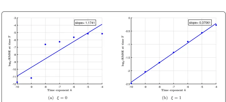
elementary_minus34 1.17 0.37 0.38 0.40 0.39 0.31
elementary_minus0.6_1 0.75 0.69 0.69 0.69 0.71 0.70
elementary4minus3 0.87 0.87 0.87 0.87 0.87 0.87
elementary1minus0.6 0.81 0.80 0.80 0.80 0.80 0.80
1Errors close to machine accuracy; no empirical convergence rate calculated (see also equation (18)).
As representatives of the class of SDEs (1), we consider here the SDEs given in Table1. In the remainder of this chapter, we present and discuss some key results of the simula-tion studies.
3.1 Key results
The empirical convergence rates obtained by the Euler scheme for the above stated step sizes=T/nwithn= 2n˜,n˜∈ {4, . . . , 10}are given in Table2(outward pointing drift
co-efficients highlighted in light gray, the discontinuity in gray). Our results show that
(i) in general, we loose convergence order one, which the Euler scheme has under standard assumptions for SDEs with additive noise,
(ii) and that a crucial factor is whether the drift coefficient is inward or outward pointing: for inward pointing coefficients the guaranteed convergence order3/4is recovered, which is not always the case for outward pointing coefficients.
(iii) Moreover, empirical convergence rates are less stable with respect to the initial value for outward pointing drift coefficients. The largest difference amounts to 0.86 for elementary_minus34.
To address the latter aspect, we supplement the numerical results for the drift coefficient elementary_minus34 by results obtained using the alternative error measureeinc(n), in-troduced in Sect.2.2. In Table3, we clearly observe that the estimate of the rate based on error incrementseinc(n) is more stable. However, the estimate is still far away from the the-oretically guaranteed convergence rate of34–εfor arbitrarily smallε> 0 for an equidistant time grid (see page 3).
im-Table 3 Empirical convergence rates, based on step sizes 2–n˜,n˜∈ {4,. . ., 10}
Initial values 0 1 1.2 1.25 1.4 2
einc(n) elementary_minus34 0.32 0.30 0.32 0.32 0.28 0.29
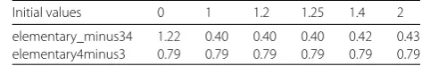
Table 4 Numerical Heun convergence rates, based on step sizes 2–n˜,n˜∈ {4,. . ., 10}
Initial values 0 1 1.2 1.25 1.4 2
elementary_minus34 1.15 0.42 0.38 0.38 0.41 0.40
elementary4minus3 0.77 0.77 0.77 0.77 0.77 0.77
Table 5 Numerical Platen convergence rates, based on step sizes 2–n˜,n˜∈ {4,. . ., 10}
Initial values 0 1 1.2 1.25 1.4 2
elementary_minus34 1.22 0.40 0.40 0.40 0.42 0.43
elementary4minus3 0.79 0.79 0.79 0.79 0.79 0.79
prove significantly, and the schemes do not yield a better resolution of the discontinuity (see Tables4and5).
3.2 Drift direction and initial value
For an outward pointing drift coefficient, the numerical convergence order even seems to depend on the initial value and the spectrum of orders obtained for different initial values is very broad with values between 0.25 and 1.17 (see Table2).
On the other hand, for an inward pointing drift coefficient, the convergence order seems to be independent of the initial value and the spectrum of orders numerically obtained for different initial values and inward pointing drift coefficients is tight with values between 0.80 and 0.91 (see Table2). The stability of the estimates is due to the ergodicity of the SDE and the Euler scheme in this case, see Sect.2.4. The geometric convergence speed in Proposition2explains why the numerical tests for inward pointing drift coefficients yield such stable estimates, independently of the initial value:Xnum
T andxnare, for a sufficiently
large number of grid pointsn+ 1, close to their unique stationary distributions, which stabilizes the Monte Carlo estimates. Also, as pointed out already above, the guaranteed convergence order 3/4 is recovered here.
For the above equations, the structure of the drift coefficient is directly related to the number of drift changes. An inward pointing drift coefficient results in many drift changes, while in the case of an outward pointing drift coefficient, only few drift changes occur. We can further observe that:
(i) when starting away from the discontinuity, numerical rates for outward pointing drift coefficients are better than for inward ones;
(ii) when starting close to the discontinuity, outward pointing drift coefficients imply worse numerical convergence rates than inward ones.
So in the latter case we obtain a positive correlation between the number of drift changes and the numerical convergence rate, which implies that frequent drift changes are not necessarily bad for the quality of the approximation—quite the contrary seems to apply, which is surprising at first glance.
on the other hand pushes the solution away from the discontinuity implying a low number of drift changes. Those rare drift changes entail the risk that an approximated path that missed a drift change in the true solution evolves in the wrong direction leading to large errors. The occurrence of drift changes and the implication for the approximated solution will be further elucidated in Sect.3.4.
3.3 Jump height
The intensity of the effects related to inward and outward pointing drift coefficients de-pends on the jump height, i.e., the distance between assigned drift values. In case of elementary_minus34, this distance amounts to 7, whereas it is 1.6 in case of elemen-tary_minus0.6_1. The empirical convergence rates in Table2 show the following: The higher the jump height, the more pronounced are the effects described in Sect. 3.2. Exemplary, there is a difference of 0.8 in the empirical convergence rates for tary_minus34 for initial values 0 and 1, whereas this difference is only 0.06 for elemen-tary_minus0.6_1. This phenomenon is related to a scaling property. By enlarging the drift value, the influence of the diffusive part of the SDE is weakened. Consider, e.g., the SDE
dXt=αsgn(Xt)dt+dWt
withα≥1. Using the new variableYt=1αXt, we have the dynamics
dYt=sgn(Yt)dt+1
αdWt,
with a reduced diffusion coefficient. So, forαlarge and initial values far away from the dis-continuity, the dynamics of the Euler scheme is almost purely deterministic, which leads to the observed higher empirical convergence rates.
3.4 Case study of an inward versus outward pointing drift coefficient
In this subsection, we analyze the pattern described in3.2in more detail, exemplary for the drift coefficients elementary4minus3 and elementary_minus34.
3.4.1 Drift changes
Figure1shows the average number of drift changes for both coefficients. The behavior goes along with the intuitive understanding described above. Here,n˜ is the exponent of the dyadic step size= 2–n˜. Note that for step sizes 2–4to 2–8and elementary_minus34 the number of drift changes stays below 2.
3.4.2 Comparison of solution sample paths
Figure2shows 100 sample paths of the numerical reference solution (= 2–14). The black line represents the discontinuity in the drift coefficient.
In the situation of Fig.2(b), where the solution drifts away from the discontinuity, it is of tremendous importance whether a drift change is captured by the approximation or not: the solution does not stay close to the discontinuity, and thus, there are not many chances for a drift correction to take place, see Fig.3. For the SDE,
dXt=α1·1(–∞,0)(Xt) +α2·1[0,∞)(Xt)
Figure 1Average number of drift changes forξ= 1.4: elementary4minus3 vs. elementary_minus34
Figure 2Comparison of solution paths: elementary4minus3 vs. elementary_minus34
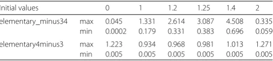
Table 6 Largest and smallest Euler errors
Initial values 0 1 1.2 1.25 1.4 2
elementary_minus34 max 0.045 1.331 2.614 3.087 4.508 0.335
min 0.0002 0.179 0.331 0.383 0.696 0.059
elementary4minus3 max 1.223 0.934 0.968 0.981 1.013 1.271
min 0.005 0.005 0.005 0.005 0.005 0.005
with α1< 0 <α2 andξ > 0 the conditional probabilityp(ξ,θ,) that the exact solution changes its drift over [0,] given that the approximationx1att=has valueθ≥0 (and thus has not changed its drift) satisfies
p(ξ,θ,) :=P
see, e.g., [11, p. 169]. So the (conditional) probability of missing drift changes is not ne-gligible and even close to one for smallξ orθ. Due to the very small probability (16) of a drift change for outward pointing drift coefficients, the empirical convergence rate might be subject to rare event simulation effects. The topic of rare events and their implications for the empirical convergence rate will be further addressed in Sect.3.5.
3.4.3 Largest error
The latter observation is also reflected in the largest distance for 104sample paths be-tween the approximation based on step size 2–10and the numerical reference solution, see Table6. The largest distances amount to 1.271 for elementary4minus3 and 4.508 for elementary_minus34.
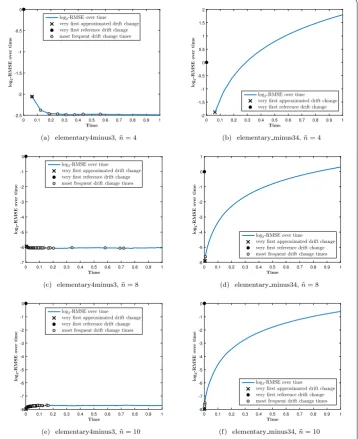
3.4.4 Evolution of the error over time
To gain even more insight, we compare the empirical RMSE for increasing timetof ele-mentary4minus3 and elementary_minus34 when starting in the discontinuityξ= 1.4 for step sizes 2–4, 2–8, and 2–10by plotting the base-2 logarithm of the RMSE against the time (see Fig.4). We have added in these figures the following additional information: If the number is not zero, the most frequent times of drift changes corresponding to the chosen step size are indicated. The number of plotted drift change times is based on the average number of drift changes over the simulated sample paths.
Furthermore, if in the corresponding cases drift changes occur, we add the very first drift change (of all simulated paths) of the numerical reference solution and the Euler schemes. They are generated by finding the time at which the first drift change occurs for 104saved paths and then taking the minimum over all that times. The time is registered as the point of discretization at which a drift change that took place was detected. The very first drift change of the reference solution is marked at a height of zero for a better distinguishability. RMSE over time and drift change times are calculated on a basis of 104simulation paths.
We can extract from Fig.4at least two features:
(i) The error stays constant or even decreases over time for elementary4minus3 in contrast to a strong error accumulation over time for elementary_minus34. (Note that the ordinate has a base-2 log scale.)
Figure 4Comparison of the error evolution over time forξ= 1.4 for different step sizes: elementary4minus3 vs. elementary_minus34
This illustrates again the stabilizing effect of an inward pointing drift coefficient and the importance of capturing the first drift changes correctly in case of an outward pointing drift coefficient.
3.4.5 Distribution of error sizes
Besides the empirical RMSE itself, the empirical distribution of the errors int=T is of interest. The error at final timeTis quantified by|xN–xn|for step size=T/n= 2–˜n. The
Figure 5Distribution of the error at timeTfor different step sizes for elementary4minus3 and elementary_minus34 withξ= 1.4
Figure 6Euler rates of convergence for elementary_minus34 forξ∈ {0, 1}
of simulated paths with an error of machine accuracy size for elementary_minus34. We will discuss this feature in more detail in the next subsection.
3.5 Rare events and goodness of the regression fit
In case of an outward pointing drift coefficient the empirical RMSE and the linear regres-sion estimates become unreliable or at least questionable.
Moreover, for an outward pointing drift coefficient, the Euler scheme and the exact so-lution coincide with high probability, which explains, e.g., the errors close to machine accuracy for the drift coefficientsignand the initial valueξ= 5. Note that in this setting the number of paths with at least one drift change is even zero over all saved 104solution paths.
To explain this phenomenon, consider again the SDE
dXt=α1·1(–∞,0)(Xt) +α2·1[0,∞)(Xt)
dt+dWt, t≥0, X0=ξ, (17)
withα1< 0 <α2. An application of formula (5.13) in Chap. 3.5.C in [17] gives
Pinf t≥0|Xt|> 0
= 1 –e2α1ξ––2α2ξ+, ξ= 0. (18)
Note that an initial valueξ= 0 is not a restriction as we analyze the case of an initial value far away from the discontinuity. So, for drift values –α1=α2= 1, and an initial valueξ= 5, the Euler scheme is exact with a probability of at least 1 –e–10≈0.99995460 . . . .
To summarize: Standard Monte Carlo simulations for testing convergence rates seem to be unreliable in the case of outward pointing coefficients. No stable asymptotic regime seems to be reached by our estimators. Smaller step sizes or a larger Monte Carlo sample might be a remedy for this problem, similar to [14] where moment explosions of the Euler scheme for SDEs with superlinear coefficients are observed in a numerically asymptotic setting. Another remedy might be the usage of a rare event simulation technique such as the one used in [43] in the context of power flow reliability, where the probability of an outage is very small. But this is beyond the scope of the present manuscript.
Instead, we supplement our numerical study of the convergence rate by numerical in-vestigations of the qualitative behavior of the Euler scheme applied to a multi-dimensional SDE with a similar structure to equation (1). Those are used in a financial market model, the so-called Atlas model, to describe the evolution of the capital distribution. Having addressed the long time properties of the Euler scheme on a theoretical basis for a partic-ular one-dimensional SDE in2.4, the aim is now to recover this aspect of the long-time behavior numerically also for a multi-dimensional SDE.
4 The Euler scheme for the Atlas model
In this section, we use the Euler scheme to simulate the so-called Atlas model, which is a particular first-order market model [4]. In such models, the asset dynamics depend on the size (measured in terms of market capitalization) of the corresponding firm, which results in an SDE model with discontinuous coefficients.
4.1 First-order market models
Afirst-order model [4] is defined as follows: Letγ,g1, . . . ,gd∈Randσ1, . . . ,σd∈(0,∞)
such that
g1< 0, g1+g2< 0, . . . , g1+· · ·+gd–1< 0, g1+· · ·+gd= 0.
Consider now stocks for which the market capitalizations are given byX1, . . . ,Xd, where the indexi∈ {1, 2, . . . ,d}indicates the name of the firm, and that follow the dynamics
Here,W1, . . . ,Wdare independent Brownian motions and the growth ratesγi: [0,∞)→R
Ties in the ranking are resolved by giving the firm with a lower indexithe better ranking. So in such a model, thekth largest firm is assigned a growth rate ofγ+gkand a volatility ofσkover the whole time horizon.
According to [4], the simplest among the first-order models is the so-calledAtlas model, which was introduced in [8, Ex. 5.3.3]. Within the setting of (19) and (20), choosing
γ =g> 0, gk= –g, k= 1, . . . ,d– 1,
gd= (d– 1)g, and σi(t) =σ> 0, i= 1, . . . ,d,
(22)
leads to the Atlas model. Here, only the smallest stock in the market—called the Atlas stock—has a nonzero but positive growth rate (for its log-dynamics).
By settingYi(t) :=logXi(t),i= 1, . . . ,d, as well as plugging in the Atlas parameters (22)
in our first-order model (19)–(20), we obtain the Atlas model in compact form as follows:
dYi(t) = (d·g)1{ri(t)=d}dt+σdWi(t), i= 1, . . . ,d. (23)
As stated in [4, Prop. 2.3], the solution of (23) satisfies the ergodic relation
lim
i.e., all stocks in the market asymptotically spent at each rank approximately the same amount of time. Similar ergodic relations also hold for general first-order market models.
4.2 Numerical results
For simulations of the Atlas and general first-order models, one has to rely on discretiza-tion schemes such as the Euler method. In this subsecdiscretiza-tion, we test whether the Euler scheme is able to recover the long time behavior (24), i.e., whether the discrete occupation rates
whereriis the discretized counterpart of (21) based on the Euler scheme andT/∈N, converge to the analytical value.
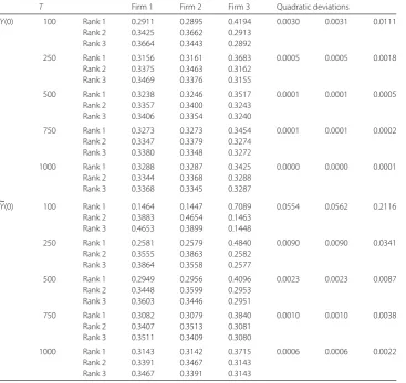
Table 7 Discrete occupation rates for the discretized Atlas model
T Firm 1 Firm 2 Firm 3 Quadratic deviations
Y(0) 100 Rank 1 0.2911 0.2895 0.4194 0.0030 0.0031 0.0111
Rank 2 0.3425 0.3662 0.2913
Rank 3 0.3664 0.3443 0.2892
250 Rank 1 0.3156 0.3161 0.3683 0.0005 0.0005 0.0018
Rank 2 0.3375 0.3463 0.3162
Rank 3 0.3469 0.3376 0.3155
500 Rank 1 0.3238 0.3246 0.3517 0.0001 0.0001 0.0005
Rank 2 0.3357 0.3400 0.3243
Rank 3 0.3406 0.3354 0.3240
750 Rank 1 0.3273 0.3273 0.3454 0.0001 0.0001 0.0002
Rank 2 0.3347 0.3379 0.3274
Rank 3 0.3380 0.3348 0.3272
1000 Rank 1 0.3288 0.3287 0.3425 0.0000 0.0000 0.0001
Rank 2 0.3344 0.3368 0.3288
Rank 3 0.3368 0.3345 0.3287
Y(0) 100 Rank 1 0.1464 0.1447 0.7089 0.0554 0.0562 0.2116
Rank 2 0.3883 0.4654 0.1463
Rank 3 0.4653 0.3899 0.1448
250 Rank 1 0.2581 0.2579 0.4840 0.0090 0.0090 0.0341
Rank 2 0.3555 0.3863 0.2582
Rank 3 0.3864 0.3558 0.2577
500 Rank 1 0.2949 0.2956 0.4096 0.0023 0.0023 0.0087
Rank 2 0.3448 0.3599 0.2953
Rank 3 0.3603 0.3446 0.2951
750 Rank 1 0.3082 0.3079 0.3840 0.0010 0.0010 0.0038
Rank 2 0.3407 0.3513 0.3081
Rank 3 0.3511 0.3409 0.3080
1000 Rank 1 0.3143 0.3142 0.3715 0.0006 0.0006 0.0022
Rank 2 0.3391 0.3467 0.3143
Rank 3 0.3467 0.3391 0.3143
volatility.bTable7presents the discrete occupation rates (averaged overM= 103 repeti-tions) for= 2–14and different values ofTas well as the sum of the squared deviations from the analytical asymptotic occupation rate. As expected, the discrete occupation rates converge to the analytical asymptotic occupation rate of 1/d= 1/3 with increasing time horizon.
Furthermore, results suggest that less varying initial capitalizations imply that the nu-merical values are closer to the analytical result already for shorter time horizons, which coincides with the intuitive understanding. We also simulated the above scenarios with
= 2–10instead of= 2–14: all occupation times were equal with an accuracy of four digits and one third of the 90 occupation rates differed in the fifth digit. This suggests that—as soon as the step size is small enough—a further refinement of the step size is no longer beneficial and the crucial simulation parameter isT, the endpoint of the considered time horizon.
5 Conclusion and outlook
that the main difficulty in measuring the empirical convergence rates is how to appropri-ately capture drift changes. For inward pointing coefficients, we obtained stable estimates, which are in accordance with the theoretical results. For outward pointing cases, the es-timates seem to be unreliable, no stabilizing asymptotic regime seems to be reached for the estimates. We tested two higher-order numerical schemes that are frequently used in a setting where coefficients are sufficiently smooth. However, both schemes did not lead to an improved behavior.
Acknowledgements
Parts of this work were carried out while A. Neuenkirch was visiting the Facultad de Matemáticas de la Universidad de Sevilla; A. Neuenkirch wishes to thank the Dpto. Ecuaciones Diferenciales y Análisis Numérico for its hospitality and support. Moreover, the authors would like to thank the referees for their insightful comments and remarks.
Funding
This work was supported by the DFG grant No. GO 1920/4-1. Moreover, the publication of this article was funded by the Ministry of Science, Research and the Arts Baden-Württemberg and the University of Mannheim.
Availability of data and materials Not applicable.
Competing interests
The authors declare that they have no competing interests.
Authors’ contributions
All authors contributed to all parts of the manuscript. All authors read and approved the final manuscript.
Endnotes
a We use the expressions “numerical” and “empirical” rate (respectively order) of convergence synonymously. b The market parameters are inspired by parameters from A. Banner’s (INTECH Investment Technologies LLC,
Princeton) presentation on “Equity Market Stability” given at the WCMF6 conference, Santa Barbara, 2014.
Publisher’s Note
Springer Nature remains neutral with regard to jurisdictional claims in published maps and institutional affiliations.
Received: 23 January 2019 Accepted: 1 October 2019
References
1. Alfonsi, A.: Strong order one convergence of a drift implicit Euler scheme: application to the CIR process. Stat. Probab. Lett.83, 602–607 (2013)
2. Asmussen, S., Taksar, M.: Controlled diffusion models for optimal dividend pay-out. Insur. Math. Econ.20, 1–15 (1997) 3. Balakrishnan, A.V.: On stochastic bang bang control. Appl. Math. Optim.6, 91–96 (1980)
4. Banner, A.D., Fernholz, R., Karatzas, I.: Atlas models of equity markets. Ann. Appl. Probab.15, 2296–2330 (2005) 5. Bayram, M., Partal, T., Orucova Buyukoz, G.: Numerical methods for simulation of stochastic differential equations. Adv.
Differ. Equ.2018, Paper No. 17 (2018)
6. Detemple, J.B., Garcia, R., Rindisbacher, M.: A Monte Carlo method for optimal portfolios. J. Finance58, 401–446 (2003)
7. Eberle, A.: Markov Processes. Lecture notes, University of Bonn (2016)
8. Fernholz, E.R.: Stochastic Portfolio Theory. Applications of Mathematics, Stochastic Modelling and Applied Probability, vol. 48. Springer, New York (2002)
9. Fernholz, R., Ichiba, T., Karatzas, I.: A second-order stock market model. Ann. Finance9, 439–454 (2013) 10. Gihman, I., Skorohod, A.: Stochastic Differential Equations. Springer, Berlin (1972)
11. Gobet, E.: Weak approximation of killed diffusion using Euler schemes. Stoch. Process. Appl.87, 167–197 (2000) 12. Gyöngy, I.: A note on Euler’s approximations. Potential Anal.8, 205–216 (1998)
13. Halidias, N., Kloeden, P.E.: A note on the Euler–Maruyama scheme for stochastic differential equations with a discontinuous monotone drift coefficient. BIT Numer. Math.48, 51–59 (2008)
14. Hutzenthaler, M., Jentzen, A., Kloeden, P.E.: Strong and weak divergence in finite time of Euler’s method for stochastic differential equations with non-globally Lipschitz continuous coefficients. Proc. R. Soc. Lond., Ser. A, Math. Phys. Eng. Sci.467, 1563–1576 (2011)
15. Ichiba, T., Papathanakos, V., Banner, A., Karatzas, I., Fernholz, R.: Hybrid Atlas models. Ann. Appl. Probab.21, 609–644 (2011)
16. Karatzas, I., Fernholz, R.: Stochastic portfolio theory: an overview. In: Handbook of Numerical Analysis, vol. 15, pp. 89–167 (2009)
17. Karatzas, I., Shreve, S.E.: Brownian Motion and Stochastic Calculus. Springer, New York (1991)
19. Kloeden, P.E., Platen, E.: Numerical Solution of Stochastic Differential Equations, vol. 23. Springer, Berlin (1999) [u.a.], corr. 3. print ed.
20. Kohatsu-Higa, A., Lejay, A., Yasuda, K.: On weak approximation of stochastic differential equations with discontinuous drift coefficient. In: Hara, C. (ed.) Mathematical Economics, Kyoto, Japan, vol. 1788, pp. 94–106 (2011)
21. Kushner, H.J., Dupuis, P.: Numerical Methods for Stochastic Control Problems in Continuous Time, 2nd edn. Applications of Mathematics (New York). Stochastic Modelling and Applied Probability, vol. 24. Springer, New York (2001)
22. LaBolle, E.M., Quastel, J., Fogg, G.E., Gravner, J.: Diffusion processes in composite porous media and their numerical integration by random walks: generalized stochastic differential equations with discontinuous coefficients. Water Resour. Res.36, 651–662 (2000)
23. Leobacher, G., Szölgyenyi, M.: A numerical method for SDEs with discontinuous drift. BIT Numer. Math.56, 151–162 (2016)
24. Leobacher, G., Szölgyenyi, M.: A strong order 1/2 method for multidimensional SDEs with discontinuous drift. Ann. Appl. Probab.27, 2383–2418 (2017)
25. Leobacher, G., Szölgyenyi, M.: Convergence of the Euler–Maruyama method for multidimensional SDEs with discontinuous drift and degenerate diffusion coefficient. Numer. Math.138, 219–229 (2018)
26. Leobacher, G., Szölgyenyi, M., Thonhauser, S.: On the existence of solutions of a class of SDEs with discontinuous drift and singular diffusion. Electron. Commun. Probab.20, Paper No. 6 (2015)
27. Mattingly, J., Stuart, A., Higham, D.: Ergodicity for SDEs and approximations: locally Lipschitz vector fields and degenerate noise. Stoch. Process. Appl.101, 185–232 (2002)
28. Meyn, S., Tweedie, R.: Markov Chains and Stochastic Stability. Springer, Berlin (1993)
29. Müller-Gronbach, T., Yaroslavtseva, L.: On the performance of the Euler–Maruyama scheme for SDEs with discontinuous drift coefficient (2018).arXiv:1809.08423
30. Neuenkirch, A., Szölgyenyi, M.: The Euler-Maruyama scheme for SDEs with irregular drift: convergence rates via reduction to a quadrature problem (2019).arXiv:1904.07784
31. Neuenkirch, A., Szölgyenyi, M., Szpruch, L.: An adaptive Euler–Maruyama scheme for stochastic differential equations with discontinuous drift and its convergence analysis. SIAM J. Numer. Anal.57, 378–403 (2019)
32. Neuenkirch, A., Szpruch, L.: First order strong approximations of scalar SDEs defined in a domain. Numer. Math.128, 103–136 (2014)
33. Ngo, H.-L., Taguchi, D.: Strong rate of convergence for the Euler–Maruyama approximation of stochastic differential equations with irregular coefficients. Math. Comput.85, 1793–1819 (2016)
34. Ngo, H.-L., Taguchi, D.: On the Euler–Maruyama approximation for one-dimensional stochastic differential equations with irregular coefficients. IMA J. Numer. Anal.37, 1864–1883 (2017)
35. Ngo, H.-L., Taguchi, D.: Strong convergence for the Euler–Maruyama approximation of stochastic differential equations with discontinuous coefficients. Stat. Probab. Lett.125, 55–63 (2017)
36. Olama, M.M., Djouadi, S.M., Charalambous, C.D.: Stochastic differential equations for modeling, estimation and identification of mobile-to-mobile communication channels. IEEE Trans. Wirel. Commun.8, 1754–1763 (2009) 37. Roberts, G.O., Tweedie, R.L.: Exponential convergence of Langevin distributions and their discrete approximations.
Bernoulli2, 341–363 (1996)
38. Shardin, A.A., Szölgyenyi, M.: Optimal control of an energy storage facility under a changing economic environment and partial information. Int. J. Theor. Appl. Finance19, 1650026 (2016)
39. Simonsen, M., Leth, J., Schiøler, H., Cornean, H.D.: A simple stochastic differential equation with discontinuous drift. In: Proceedings Third International Workshop on Hybrid Autonomous Systems, HAS 2013, Rome, Italy, 17th March 2013, pp. 109–123 (2013)
40. Simonsen, M., Schioler, H., Leth, J., Cornean, H.: A convergence result for the Euler–Maruyama method for a simple stochastic differential equation with discontinuous drift. In: 2014 American Control Conference, pp. 5180–5185 (2014)
41. Touzi, N.: Optimal Stochastic Control, Stochastic Target Problems, and Backward SDE. Fields Institute Monographs, vol. 29. Springer, New York; Fields Institute for Research in Mathematical Sciences, Toronto, ON. With Chap. 13 by Angès Tourin (2013)
42. Veretennikov, A.J.: On strong solutions and explicit formulas for solutions of stochastic integral equations. Math. USSR Sb.39, 387–403 (1981)
43. Wadman, W.S., Crommelin, D.T., Zwart, B.P.: A large-deviation-based splitting estimation of power flow reliability. ACM Trans. Model. Comput. Simul.26, 1–26 (2016)