Daniel J. Bernstein1,2 and Tanja Lange2
1 Department of Computer Science
University of Illinois at Chicago Chicago, IL 60607–7045, USA
2 Department of Mathematics and Computer Science
Technische Universiteit Eindhoven
P.O. Box 513, 5600 MB Eindhoven, The Netherlands
Abstract. This paper shows, assuming standard heuristics regarding
the number-field sieve, that a “batch NFS” circuit of area L1.181...+o(1)
factorsL0.5+o(1)separateB-bit RSA keys in timeL1.022...+o(1). HereL=
exp((log 2B)1/3(log log 2B)2/3). The circuit’s area-time product
(price-performance ratio) is justL1.704...+o(1) per key. For comparison, the best
area-time product known for a single key isL1.976...+o(1).
This paper also introduces new “early-abort” heuristics implying that “early-abort ECM” improves the performance of batch NFS by a
super-polynomial factor, specifically exp((c+ o(1))(log 2B)1/6(log log 2B)5/6)
where c is a positive constant.
Keywords:integer factorization, number-field sieve, price-performance ratio, batching, smooth numbers, elliptic curves, early aborts
1
Introduction
The cryptographic community reached consensus a decade ago that a 1024-bit RSA key can be broken in a year by an attack machine costing significantly less
than 109 dollars. See [51], [38], [24], and [23]. The attack machine is an
opti-mized version of the number-field sieve (NFS), a factorization algorithm that has
been intensively studied for twenty years, starting in [36]. The run-time
analy-sis of NFS relies on various heuristics, but these heuristics have been confirmed in a broad range of factorization experiments using several independent NFS
software implementations: see, e.g., [29], [30], [31], and [4].
Despite this threat, 1024-bit RSA remains the workhorse of the Internet’s “DNS Security Extensions” (DNSSEC). For example, at the time of this writing
(November 2014), the IP address of the domain dnssec-deployment.org is
• signed by that domain’s 1024-bit “zone-signing key”, which in turn is
This work was supported by the National Science Foundation under grant 1018836 and by the Netherlands Organisation for Scientific Research (NWO) under grant
639.073.005. Permanent ID of this document:4f99b1b911984e501c099f514d8fd2ce.
2 Daniel J. Bernstein and Tanja Lange
• signed by that domain’s 2048-bit “key-signing key”, which in turn is
• signed by .org’s 1024-bit zone-signing key, which in turn is
• signed by .org’s 2048-bit key-signing key, which in turn is
• signed by the DNS root’s 1024-bit zone-signing key, which in turn is
• signed by the DNS root’s 2048-bit key-signing key.
An attacker can forge this IP address by factoring any of the three 1024-bit RSA keys in this chain.
A report [41] last year indicated that, out of the 112 top-level domains using
DNSSEC, 106 used the same key sizes as .org. We performed our own survey
of zone-signing keys in September 2014, after many new top-level domains were added. We found 286 domains using 1024-bit keys; 4 domains using 1152-bit keys; 192 domains using 1280-bit keys; and just 22 domains using larger keys.
Almost all of the 1280-bit keys are for obscure domains such as .boutiqueand
.rocks; high-volume domains practically always use 1024-bit keys.
Evidently DNSSEC users find the attacks against 1024-bit RSA less worrisome than the obvious costs of moving to larger keys. There are, according to our informal surveys of these users, three widespread beliefs supporting the use of 1024-bit RSA:
• A typical RSA key is believed to be worth less than the cost of the attack
machine.
• Building the attack machine means building a huge farm of
application-specific integrated circuits (ASICs). Standard computer clusters costing the same amount of money are believed to take much longer to perform the same calculations.
• It is believed that switching RSA signature keys after (e.g.) a month will
render the attack machine useless, since the attack machine requires a full year to run.
Consider, for example, the following quote from the latest “DNSSEC operational
practices” recommendations [32, Section 3.4.2], published December 2012:
DNSSEC signing keys should be large enough to avoid all known crypto-graphic attacks during the effectivity period of the key. To date, despite huge efforts, no one has broken a regular 1024-bit key; in fact, the best completed attack is estimated to be the equivalent of a 700-bit key. An attacker breaking a 1024-bit signing key would need to expend phenom-enal amounts of networked computing power in a way that would not be detected in order to break a single key. Because of this, it is estimated that most zones can safely use 1024-bit keys for at least the next ten years.
1.1. Contents of this paper.This paper analyzes theasymptotic cost,
specif-ically the price-performance ratio, of breaking many RSA keys. We emphasize
several words here:
• “Many”: The attacker is faced not with a single target, but with many
tar-gets. The algorithmic task here is not merely to break, e.g., a single 1024-bit RSA key; it is to break more than two hundred 1024-1024-bit RSA keys for DNSSEC top-level domains, many more 1024-bit RSA keys at lower levels
of DNSSEC, millions of 1024-bit RSA keys in SSL (as in [25] and [35]; note
that upgrading SSL to 2048-bit RSA does nothing to protect the confiden-tiality of previously recorded SSL traffic), etc. This is important if there are ways to share attack work across the keys.
• “Price-performance ratio”: As in [53], [18], [50], [15], [54], [7], [51], [56],
[23], [24], etc., our main interest is not in the number of “operations” carried
out by an algorithm, but in the actual price and performance of a machine carrying out those operations. Parallelism increases price but often improves performance; large storage arrays are a problem for both price and perfor-mance. We use price-performance ratio as our primary cost metric, but we also report time separately since signature-key rotation puts a limit upon time.
• “Asymptotic”: The cost improvements that we present are superpolynomial
in the size of the numbers being factored. We thus systematically suppress all polynomial factors in our cost analyses, simplifying the analyses.
This paper presents a new “batch NFS” circuit of area L1.181...+o(1) that,
assuming standard NFS heuristics, factors L0.5+o(1) separate B-bit RSA keys
in total time just L1.022...+o(1). The area-time product is L1.704...+o(1) for each
key; i.e., the price-performance ratio is L1.704...+o(1). Here (as usual for NFS) L
means exp((logN)1/3(log logN)2/3) where N = 2B.
For comparison (see Table 1.4), the best area-time product known for factoring
a single key (without quantum computers) is L1.976...+o(1), even if non-uniform
precomputations such as Coppersmith’s “factorization factory” are allowed. The literature is reviewed below.
This paper also looks more closely at theLo(1). The main bottleneck in batch
NFS is not traditional sieving, but rather low-memory smoothness detection, mo-tivating new attention to the complexity of low-memory smoothness detection.
Traditional ECM, the elliptic-curve method of recognizing y-smooth integers,
works in low memory and takes time exp(p(2 +o(1))logylog logy). One can
reasonably guess that, compared to traditional ECM, “early-abort ECM” saves a subexponential factor here, but the complexity of early-abort ECM has never been analyzed. Section 3 of this paper introduces new early-abort heuristics
implying that the cost of early-abort ECM is expq 89 +o(1)logylog logy.
Using early aborts increases somewhat the number of auxiliary integers that need to be factored, producing a further increase in cost, but the cost is outweighed by the faster factorization.
The ECM cost is obviously bounded by Lo(1): more precisely, the cost is
4 Daniel J. Bernstein and Tanja Lange
This cost is invisible at the level of detail ofL1.704...+o(1). The speedup from ECM
to early-abort ECM is nevertheless superpolynomial and directly translates into the same speedup in batch NFS.
1.2. Security consequences.We again emphasize that our results are
asymp-totic. This prevents us from directly drawing any conclusions about 1024-bit RSA, or 2048-bit RSA, or any other specific RSA key size. Our results are nev-ertheless sufficient to undermine all three of the beliefs described above:
• Users comparing the value of an RSA key to the cost of an attack machine
need to know the per-key cost of batch NFS. This has not been seriously
studied. What the literature has actually studied in detail is the cost of NFS
attacking one key at a time; this is not the same question. Our asymptotic
results do not rule out the possibility that these costs are the same for 1024-bit RSA, but there is also no reason to be confident about any such possibility.
• Most of the literature on single-key NFS relies heavily on operations that —
for large key sizes — are not handled efficiently by current CPUs and that become much more efficient on ASICs: consider, for example, the routing
circuit in [51]. Batch NFS relies much more heavily on massively parallel
elliptic-curve scalar multiplication, exactly the operation that is shown in
[12], [11], and [17] to fit very well into off-the-shelf graphics cards. The
literature supports the view that off-the-shelf hardware is much less cost-effective than ASICs for single-key NFS, but there is no reason to think that the same is true for batch NFS.
• The natural machine size for batch NFS (i.e., the circuit area if
price-performance ratio is optimized) is larger than the natural machine size for
single-key NFS, but the naturaltime is considerably smaller. As above, these
asymptotic results undermine any confidence that one can obtain from com-paring the natural time for single-key NFS to the rotation interval for sig-nature keys: there is no reason to think that the latency of batch NFS will be as large as the latency of single-key NFS. Note that, even though this pa-per emphasizes optimal price-pa-performance ratio for simplicity, there are also techniques to further reduce the time below the natural time, hitting much lower latency targets without severely compromising price-performance ra-tio: in particular, for the core sorting subroutines inside linear algebra, one
can replace time T with T /f at the expense of replacing area A with Af2.
The standard measure of security is the total cost of attacking one key. For
example, this is what NIST is measuring in [6] when it reports “80-bit security”
for 1024-bit RSA, “112-bit security” for 2048-bit RSA, “128-bit security” for 3072-bit RSA, etc. What batch NFS illustrates is that, when there are many
user keys, the attacker’s cost per key can be smaller than the attacker’s total
cost for one key. It is much more informative to measure the attacker’s total
cost of attacking U user keys, as a function of U. It is even more informative
to measure the attacker’s chance of breaking exactly K out ofU simultaneously
There are many other examples of cryptosystems where the attack cost does not grow linearly with the number of targets. For example, it is well known
that exhaustive search finds preimages for U hash outputs in about the same
time as a preimage for a single hash output; furthermore, the first preimage that
it finds appears after only 1/U of the total time, reducing actual security by
lgU bits. However, most cryptosystems have moved up to at least a “128-bit”
security level, giving them a buffer against losing some bits of security. RSA is an exception: its poor performance at high security levels has kept it at a bleeding-edge “80-bit security” level. Even when users can be convinced to move
away from 1024-bit keys, they normally move to ≤2048-bit keys. We question
whether it is appropriate to view 1024-bit keys as “80-bit” security and 2048-bit
keys as “112-bit” security if the attacker’s costs per key are not so high.
1.3. Previous work. In the NFS literature, as in the algorithm literature in
general, there is a split between traditional analyses of “operations” (adding two
64-bit integers is one “operation”; looking up an element of a 264-byte array is one
“operation”) and modern analyses of more realistic models of computation. We
follow the terminology of our paper [14]: the “RAM metric” counts traditional
operations, while the “AT metric” multiplies the area of a circuit by the time
taken by the same circuit.
Buhler, H. Lenstra, and Pomerance showed in [19] (assuming standard NFS
heuristics, which we now stop mentioning) that NFS factors a single keyN with
RAM cost L1.922...+o(1). As above, L means exp((log 2B)1/3(log log 2B)2/3) if N
has B bits. This exponent 1.922. . .is the most frequently quoted cost exponent
for NFS.
Coppersmith in [20] introduced two improvements to NFS. The first,
“mul-tiple number fields”, reduces the exponent 1.922. . .+o(1) to 1.901. . .+o(1).
The second, the “factorization factory”, is anon-uniform algorithm that reduces
1.901. . .+o(1) to just 1.638. . .+o(1). Recall that (size-)non-uniform algorithms
are free to perform arbitrary amounts of precomputation as functions of thesize
of the input, i.e., the number of bits ofN. A closer look shows that Coppersmith’s
precomputation costs L2.006...+o(1), so if it is applied to more than L0.368...+o(1)
inputs then the precomputation cost can quite reasonably be ignored.
Essentially all of the subsequent NFS literature has consisted of analysis and
optimization of algorithms that cost L1.922...+o(1), such as the algorithm of [19].
The ideas of [20] have been dismissed for three important reasons:
• The bottleneck in [19] is sieving, while the bottleneck in [20] is ECM. Both
of these algorithms use Lo(1) operations in the RAM metric, but the o(1) is
considerably smaller for sieving than for ECM.
• Even if the o(1) in [20] were as small as theo(1) in [19], there would not be
much benefit in 1.901. . .+o(1) compared to 1.922. . .+o(1). For example,
(250)1.922 ≈296 while (250)1.901 ≈295.
• The change from 1.901. . .+o(1) to 1.638. . .+o(1) is much larger, but it
comes at the cost of massive memory consumption. Specifically, [20] requires
spaceL1.638...+o(1), while [19] uses space justL0.961...+o(1). This is not visible
6 Daniel J. Bernstein and Tanja Lange
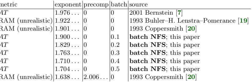
metric exponent precomp batch source
AT 1.976. . . 0 0 2001 Bernstein [7]
RAM (unrealistic) 1.922. . . 0 0 1993 Buhler–H. Lenstra–Pomerance [19]
RAM (unrealistic) 1.901. . . 0 0 1993 Coppersmith [20]
AT 1.900. . . 0 0.1 batch NFS; this paper
AT 1.829. . . 0 0.2 batch NFS; this paper
AT 1.763. . . 0 0.3 batch NFS; this paper
AT 1.710. . . 0 0.4 batch NFS; this paper
AT 1.704. . . 0 0.5 batch NFS; this paper
RAM (unrealistic) 1.638. . . 2.006. . . 0 1993 Coppersmith [20]
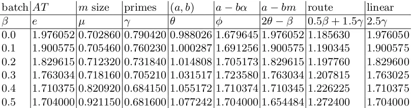
Table 1.4. Asymptotic exponents for several variants of NFS, assuming standard
heuristics. “Exponent” emeans asymptotic cost Le+o(1) per key factored. “Precomp”
2θmeans that there is a precomputation involving integer pairs (a, b) up toLθ+o(1), for
total precomputation cost L2θ+o(1); algorithms without precomputation have 2θ = 0.
“Batch” β means batch size Lβ+o(1); algorithms handling each key separately have
β = 0. See Section 2 for further details.
increasingly severe as computations grow larger. As a concrete illustration
of the real-world costs of storage and computation, paying for 270 bytes of
slow storage (about 30·109 USD in hard drives) is much more troublesome
than paying for 280 floating-point multiplications (about 0.02·109 USD in
GPUs plus 0.005·109 USD for a year of electricity).
We quote A. Lenstra, H. Lenstra, Manasse, and Pollard [37]: “There is no
indi-cation that the modifiindi-cation proposed by Coppersmith has any practical value.” At the time there was already more than a decade of literature showing how to analyze algorithm asymptotics in more realistic models of computation that
ac-count for memory consumption, communication, etc.; see, e.g., [18]. Bernstein in
[7] analyzed the circuit performance of NFS, concluding that an optimized circuit
of area L0.790...+o(1) would factor N in time L1.18...+o(1), for price-performance
ratio L1.976...+o(1). [7] did not analyze the factorization factory but did analyze
multiple number fields, concluding that they did not reduce AT cost. The gap
between the RAM exponent 1.901. . . +o(1) from [20] and the AT exponent
1.976. . .+o(1) from [7] is explained primarily by communication overhead in-side linear algebra, somewhat moderated by parameter choices that reduce the cost of linear algebra at the expense of relation collection.
We pointed out in [14] that the factorization factory does not reduce AT
cost. In Section 2 we review the reason for this and explain how batch NFS
works around it. We also presented in [14] a superpolynomial improvement to
the factorization factory in the RAM metric, by eliminating ECM in favor of
2
Exponents
This section reviews NFS and then explains how to drastically reduce the AT
cost of NFS through batching. The resulting cost exponent, 1.704. . .in Table 1.4,
is new. All costs in this section are expressed as Le+o(1) for various exponentse.
Section 3 looks more closely at the Lo(1) factor.
2.1. QS: the quadratic sieve (1982).As a warmup for NFS we briefly review
the general idea of combining congruences, using QS as an example.
QS writes down a large collection of congruences modulo the target integer
N and tries to find a nontrivial subcollection whose product is a congruence of
squares. One can then reasonably hope that the difference of square roots has a
nontrivial factor in common withN.
Specifically, QS computes s ≈ √N and writes down the congruences s2 ≡
s2−N, (s+ 1)2 ≡(s+ 1)2−N, etc. The left side of each congruence is already a
square. The main problem is to find a nontrivial set of integers a such that the
product of (s+a)2−N is a square.
If (s+a)2 −N is divisible by a very large prime then it is highly unlikely
to participate in a square: the prime would have to appear a second time. QS
therefore focuses onsmoothcongruences: congruences where (s+a)2−N factors
completely into small primes. Applying linear algebra modulo 2 to the matrix of exponents in these factorizations is guaranteed to find nonempty subsets of the congruences with square product once the number of smooth congruences exceeds the number of small primes.
The integersa such that (s+a)2 −N is divisible by a prime p form a small
number of arithmetic progressions modulop. “Sieving” means jumping through
these arithmetic progressions to mark divisibility, the same way that the sieve of Eratosthenes jumps through arithmetic progressions to mark non-primality.
2.2. NFS: the number-field sieve (1993). NFS applies the same idea, but
instead of congruences moduloN it uses congruences modulo a related algebraic
number m−α. This algebraic number is chosen to have norm N (divided by
a certain denominator shown below), and one can reasonably hope to obtain a
factorization ofN by obtaining a random factorization of this algebraic number.
Specifically, NFS chooses a positive integer m, and writes N as a polynomial
in radixm, namelyN =f(m) wheref is a degree-dpolynomial with coefficients
fd, fd−1, . . . , f0 ∈ {0,1, . . . , m−1}. It is not difficult to see that optimizing NFS
requiresdto grow slowly withN, somis asymptotically on a much smaller scale
than N, although not as small as L. More precisely, NFS takes
m∈exp((µ+o(1))(logN)2/3(log logN)1/3)
where µ is a positive real constant, optimized below. Note that the inequalities
md ≤N < md+1 imply
d ∈(1/µ+o(1))(logN)1/3(log logN)−1/3.
Iff is reducible then its factorization is easy to compute and (forN reasonably
8 Daniel J. Bernstein and Tanja Lange
from now on thatf is irreducible. Define α as a root off. The norm of a−bαis
then fdad +fd−1ad−1b+· · ·+f0bd (divided by fd), and in particular the norm
of m−α is N (again divided by fd).
NFS uses the congruences a−bm ≡ a−bα modulo m−α. There are now
two numbers, a−bm and a −bα, that both need to be smooth. Smoothness
of the algebraic number a −bα is defined as smoothness of the (scaled) norm
fdad+fd−1ad−1b+· · ·+f0bd, and smoothness of an integer is defined as having
no prime divisors larger than y. Here y ∈ Lγ+o(1) is another parameter chosen
by NFS; γ >1/(6µ) is another real constant, optimized below.
The range of pairs (a, b) searched for smooth congruences is the set of coprime
integer pairs in the rectangle [−H, H]×[1, H]. HereH is chosen so that there will
be enough smooth congruences to produce squares at the end of the algorithm.
Standard heuristics state thata−bmhas smoothness probabilityL−µ/(3γ)+o(1) if
aandbare on much smaller scales thanm; in particular, ifH ∈Lθ+o(1) for some
positive real number θ then the number of congruences with a−bm smooth is
Lφ+o(1) withφ= 2θ−µ/(3γ). Standard heuristics also provide the simultaneous
smoothness probability of a−bm and a−bα, implying that to obtain enough
smooth congruences one can take H ∈Lθ+o(1) with θ = (3µγ2+ 2µ2)/(6µγ−1)
andφ= (18µγ3+ 6µ2γ+µ)/(18µγ2−3γ). See, e.g., [19]. We henceforth assume
these formulas for θ and φ in terms of µ and γ.
2.3. RAM cost analysis (1993). Sieving for y-smoothness of H2+o(1)
poly-nomial values uses H2+o(1) operations, provided that y is bounded by H2+o(1).
The point here is that the pairs (a, b) with congruences divisible by p form a
small number of shifted lattices of determinant p, usually with basis vectors of
length O(√p), making it easy to find all the lattice points inside the rectangle
[−H, H]×[1, H]. The number of operations is thus essentially the number of
points marked, and each point is marked just P
p≤y1/p≈log logy times.
Sparse techniques for linear algebra involve y1+o(1) matrix-vector
multiplica-tions, each involving y1+o(1) operations, for a total of y2+o(1) operations. Other
subroutines in NFS take negligible time, so the overall RAM cost of NFS is
Lmax{2θ,2γ}+o(1).
It is not difficult to see that the exponent max{2θ,2γ} achieves its
mini-mum value (64/9)1/3 = 1.922. . . with µ = (1/3)1/3 = 0.693. . . and θ = γ =
(8/9)1/3 = 0.961. . .. This exponent 1.922. . .is the NFS exponent from [19], and as mentioned earlier is the most frequently quoted NFS exponent. We do not
review the multiple-number-fields improvement to 1.901. . . from [20]; as far as
we know, multiple number fields do not improve any of the exponents analyzed below.
2.4. AT cost analysis (2001). In the AT metric there is an important
ob-stacle to cost H2+o(1) for sieving: namely, communicating across area H2+o(1)
takes time at least H1+o(1). One can efficiently split the sieving problem into
H2+o(1)/y1+o(1) tasks, running one task after another on a smaller array of size
y1+o(1), but communicating across this array still takes time at least y0.5+o(1),
Fortunately, there is a much more efficient alternative to sieving: ECM,
ex-plained in Appendix A. What matters in this section is that ECM tests y
-smoothness in time yo(1) on a circuit of area yo(1). A parallel array of ECM
units, each handling a separate number, tests y-smoothness of H2+o(1)
poly-nomial values in time H2+o(1)/y1+o(1) on a circuit of area y1+o(1), achieving
AT =H2+o(1).
Unfortunately, the same obstacle shows up again for linear algebra, and this time there is no efficient alternative. Multiplying a sparse matrix by a vector
requires timey0.5+o(1) on a circuit of areay1+o(1), and must be repeatedy1+o(1)
times. The overall AT cost of NFS is Lmax{2θ,2.5γ}+o(1).
The exponent max{2θ,2.5γ} achieves its minimum value 1.976. . . with µ =
0.702. . ., γ = 0.790. . ., and θ = 0.988. . .. This exponent 1.976. . . is the NFS
exponent from [7]. Notice that γ is much smaller here than it was in the RAM
optimization:yhas been reduced to keep the cost of linear algebra under control,
but this also forced θ to increase.
2.5. The factorization factory (1993). Coppersmith in [20] precomputes
“tables which will be useful for factoring any integers in a large range . . . after
the precomputation, an individual integer can be factored in timeL[1/3,1.639]”,
i.e., L≈1.639+o(1).
Coppersmith’s table is simply the set of (a, b) such thata−bm is smooth. One
reuses m, and thus this table, for any integerN between (e.g.) md and md+1.
Coppersmith’s method to factor “an individual integer” is to test smoothness
of a−bα for each (a, b) in the table. At this point Coppersmith has found the
same smooth congruences as conventional NFS, and continues with linear algebra in the usual way.
Coppersmith uses ECM to test smoothness. The problem with sieving here
is not efficiency, as in the (subsequent) paper [7], but functionality: sieving can
handle polynomial values only at regularly spaced inputs, and the pairs (a, b) in
this table are not regularly spaced.
Recall that the size of this table is Lφ+o(1) with φ= 2θ−µ/(3γ). ECM uses
Lo(1) operations per number, for a total smoothness cost of Lφ+o(1),
asymptoti-cally a clear improvement over the L2θ+o(1) for conventional NFS.
The overall RAM cost of the factorization factory is Lmax{φ,2γ}+o(1). The
exponent achieves its minimum value 1.638. . . withµ= 0.905. . .,γ = 0.819. . .,
θ = 1.003. . ., and φ= 1.638. . .. This is the exponent from [20].
The AT metric tells a completely different story, as we pointed out in [14].
The area required for the table is Lφ+o(1). This area is easy to reuse for very
fast parallel smoothness detection, finishing in time Lo(1). Unfortunately,
col-lecting the smooth results then takes time L0.5φ+o(1), for an AT cost of at least
Lmax{1.5φ,2.5γ}+o(1), never mind the problem of matching the table area with the
linear-algebra area. The minimum exponent here is above 2.4.
2.6. Batch NFS (new).We drastically reduceAT cost by sharing work across
many N’s in a different way: we process a batch of N’s in parallel, rather than
performing precomputation to be used for one N at a time. We dynamically
10 Daniel J. Bernstein and Tanja Lange
Generate (a, b). Generate (a, b). Generate (a, b). Generate (a, b). Isa−bm Isa−bm Isa−bm Isa−bm
smooth? smooth? smooth? smooth? If so, store. If so, store. If so, store. If so, store.
Repeat. Repeat. Repeat. Repeat. Generate (a, b). Generate (a, b). Generate (a, b). Generate (a, b).
Isa−bm Isa−bm Isa−bm Isa−bm smooth? smooth? smooth? smooth? If so, store. If so, store. If so, store. If so, store.
Repeat. Repeat. Repeat. Repeat. Generate (a, b). Generate (a, b). Generate (a, b). Generate (a, b).
Isa−bm Isa−bm Isa−bm Isa−bm smooth? smooth? smooth? smooth? If so, store. If so, store. If so, store. If so, store.
Repeat. Repeat. Repeat. Repeat. Generate (a, b). Generate (a, b). Generate (a, b). Generate (a, b).
Isa−bm Isa−bm Isa−bm Isa−bm smooth? smooth? smooth? smooth? If so, store. If so, store. If so, store. If so, store.
Repeat. Repeat. Repeat. Repeat.
Generate (a, b). Generate (a, b). Generate (a, b). Generate (a, b).
Isa−bm Isa−bm Isa−bm Isa−bm
smooth? smooth? smooth? smooth?
If so, store. If so, store. If so, store. If so, store.
Repeat. Repeat. Repeat. Repeat.
Generate (a, b). Generate (a, b). Generate (a, b). Generate (a, b).
Isa−bm Isa−bm Isa−bm Isa−bm
smooth? smooth? smooth? smooth?
If so, store. If so, store. If so, store. If so, store.
Repeat. Repeat. Repeat. Repeat.
Generate (a, b). Generate (a, b). Generate (a, b). Generate (a, b).
Isa−bm Isa−bm Isa−bm Isa−bm
smooth? smooth? smooth? smooth?
If so, store. If so, store. If so, store. If so, store.
Repeat. Repeat. Repeat. Repeat.
Generate (a, b). Generate (a, b). Generate (a, b). Generate (a, b).
Isa−bm Isa−bm Isa−bm Isa−bm
smooth? smooth? smooth? smooth?
If so, store. If so, store. If so, store. If so, store.
Repeat. Repeat. Repeat. Repeat.
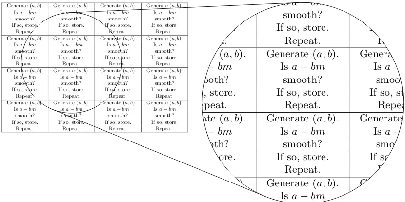
Fig. 2.7. Relation-search mesh finding pairs (a, b) where a− bm is smooth. The
following exponents are optimized for factoring a batch of L0.5+o(1) B-bit
inte-gers: The mesh has height L0.25+o(1), width L0.25+o(1), and area L0.5+o(1). The
mesh consists of L0.5+o(1) small parallel processors (illustration contains 16). Each
processor has area Lo(1). Each processor knows the same m ∈ exp((0.92115 +
o(1))(log 2B)2/3(log log 2B)1/3). Each processor generates its own L0.200484+o(1) pairs
(a, b), where a and b are bounded by L1.077242+o(1). Each processor tests each of its
own a−bm for smoothness using ECM, using smoothness bound L0.681600+o(1).
To-gether the processors generate L0.700484+o(1) separate pairs (a, b), of which L0.25+o(1)
havea−bmsmooth.
the N’s in the batch, and remove each pair as soon as possible, rather than
storing a complete table of the pairs. To avoid excessive communication costs we completely reorganize data in the middle of the computation: at the beginning
each N is repeated many times to bring N close to the pairs (a, b), while at the
end the pairs (a, b) relevant to eachN are moved much closer together. The rest
of this subsection presents the details of the algorithm.
Consider as input a batch ofLβ+o(1) simultaneous targetsN within the large
range described above. We requireβ ≤min{2φ−2γ,4θ−2φ}; if there are more
targets available at once then we actually process those targets in batches of size
Lmin{2φ−2γ,4θ−2φ}+o(1), storing no data between runs.
Consider a square mesh of Lβ+o(1) small parallel processors. This mesh is
large enough to store all of the targets N. Use each processor in parallel to test
smoothness of a−bm for L2θ−φ−0.5β+o(1) pairs (a, b) using ECM; by hypothesis
2θ − φ−0.5β ≥ 0. The total number of pairs here is L2θ−φ+0.5β+o(1). Each
smoothness test takes time Lo(1). Overall the mesh takes time L2θ−φ−0.5β+o(1)
and produces a total ofL0.5β+o(1) pairs (a, b) witha−bm smooth, i.e., onlyLo(1)
pairs for each column of the mesh. See Figure 2.7.
Isa−bα1 Isa−bα2 Isa−bα3 Isa−bα4 smooth? smooth? smooth? smooth? If so, store. If so, store. If so, store. If so, store. Send (a, b) right. Send (a, b) right. Send (a, b) right. Send (a, b) down.
Repeat. Repeat. Repeat. Repeat. Isa−bα5 Isa−bα6 Isa−bα7 Isa−bα8
smooth? smooth? smooth? smooth? If so, store. If so, store. If so, store. If so, store. Send (a, b) up. Send (a, b) left. Send (a, b) left. Send (a, b) left.
Repeat. Repeat. Repeat. Repeat. Isa−bα9 Isa−bα10 Isa−bα11 Isa−bα12
smooth? smooth? smooth? smooth? If so, store. If so, store. If so, store. If so, store. Send (a, b) right. Send (a, b) right. Send (a, b) right. Send (a, b) down.
Repeat. Repeat. Repeat. Repeat. Isa−bα13 Isa−bα14 Isa−bα15 Isa−bα16
smooth? smooth? smooth? smooth? If so, store. If so, store. If so, store. If so, store. Send (a, b) up. Send (a, b) left. Send (a, b) left. Send (a, b) left.
Repeat. Repeat. Repeat. Repeat.
smooth? smooth? smooth? smooth?
If so, store. If so, store. If so, store. If so, store. Send (a, b) right. Send (a, b) right. Send (a, b) right. Send (a, b) down.
Repeat. Repeat. Repeat. Repeat.
Isa−bα5 Isa−bα6 Isa−bα7 Isa−bα8
smooth? smooth? smooth? smooth?
If so, store. If so, store. If so, store. If so, store. Send (a, b) up. Send (a, b) left. Send (a, b) left. Send (a, b) left.
Repeat. Repeat. Repeat. Repeat.
Isa−bα9 Isa−bα10 Isa−bα11 Isa−bα12
smooth? smooth? smooth? smooth?
If so, store. If so, store. If so, store. If so, store. Send (a, b) right. Send (a, b) right. Send (a, b) right. Send (a, b) down.
Repeat. Repeat. Repeat. Repeat.
Isa−bα13 Isa−bα14 Isa−bα15 Isa−bα16
smooth? smooth? smooth? smooth?
If so, store. If so, store. If so, store. If so, store. Send (a, b) up. Send (a, b) left. Send (a, b) left. Send (a, b) left.
Repeat. Repeat. Repeat. Repeat.
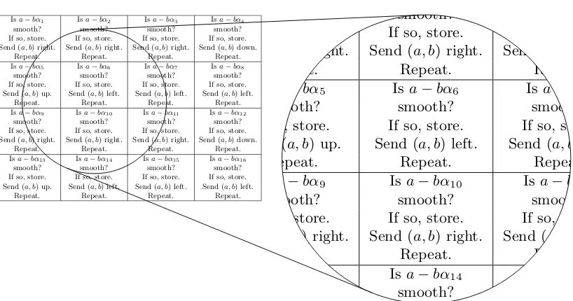
Fig. 2.8. Relation-search mesh from Figure 2.7, now finding pairs (a, b) where both
a−bm and a−bαi are smooth. For a batch of L0.5+o(1) B-bit integers: The mesh
knowsL0.25+o(1) pairs (a, b) witha−bmsmooth from Figure 2.7. Each (a, b) is copied
L0.25+o(1)times (2 times in the illustration) so that it appears in the first two rows, the
next two rows, etc. Each (a, b) visits each mesh position withinL0.25+o(1)steps (8 steps
in the illustration). Each processor knows its own targetNi and the correspondingαi,
and in each step tests each a−bαi for smoothness using ECM. Together Figure 2.7
and Figure 2.8 take timeL0.25+o(1) to search L0.700484+o(1) pairs (a, b).
from [50], taking time L0.5β+o(1). Then broadcast each pair to its entire column,
taking time L0.5β+o(1). Actually, it will suffice for each pair to appear once
somewhere in the first two rows, once somewhere in the next two rows, etc. Now consider a pair at the top-left corner. Send this pair to its right until it reaches the rightmost column, then down one row, then repeatedly to its left, then back up. In parallel move all the other elements in the first two rows on the same path. In parallel do the same for the third and fourth rows, the fifth
and sixth rows, etc. Overall this takes time L0.5β+o(1).
Observe that each pair has now visited each position in the mesh. When a
pair (a, b) visits a mesh position holding a targetN, use ECM to check whether
a−bα is smooth, taking time Lo(1). The total time to check all L0.5β+o(1) pairs
against all Lβ+o(1) targets is just L0.5β+o(1), plus the time L2θ−φ−0.5β+o(1) to
generate the pairs in the first place. See Figure 2.8.
Repeat this entire procedure Lφ−γ−0.5β+o(1) times; by hypothesis φ− γ −
0.5β ≥0. This covers a total ofL2θ−γ+o(1) pairs (a, b), of which Lφ−γ+o(1) have
a−bm smooth, so for each N there are Lo(1) pairs (a, b) for which a−bm and
a−bαare both smooth. The total number of smooth congruences found this way
across all N is Lβ+o(1). Store each smooth congruence as (N, a, b); all of these
together fit into a mesh of areaLβ+o(1). The time spent isLmax{φ−γ,2θ−γ−β}+o(1).
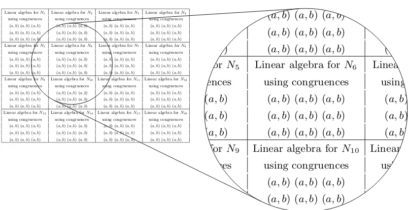
Build Lγ+o(1) copies of the same mesh, all operating in parallel, for a total