SIB MATING WITH TWO LINKED LOCI

(1)

SIB MATING WITH T W O LINKED LOCI'

C CLARK COCKERHAM A N D B. S W E I R 2

Department of Experimental Statistics, North Carolina State Uniuersity, Raleigh, N.C

Received February 5 , 1968

mating with one locus has beeii studied extensively by several authors. "!&RIGHT (1921) in terms of the correlation between uniting gametes, HAL- DANE (1937) using a generation matrix for the six possible mating types, and MALECOT (1948) using probability arguments, all produced the same recurrence relation of a measure of the degree of homozygosity, the inbreeding coefficient.

FISHER (1949) continued the generation matrix approach and found the geno- typic array after n generations of sib mating.

When several linked loci are considered, the problem of establishing a measure of the amount of inbreeding 'which lends itself readily to evaluation in all generations is more difficult. HALDANE and WADDINGTON (1931) reckoned with one hundred mating types for two alleles a t each of two loci, and found the final frequency of crossover zygotes. HALDANE (1949) extended the inbreeding coefficient to two loci, and gave its value for the offspring of full sibs from unrelated, outbred parents (the first generation of inbreeding). BENNETT (1954) returned to the generation matrix approach, restricting himself to two alleles and the nine mating tx-pes that gwie offspring heterozygous a t both loci, and listed numerical values of the dominant root of the matrix. SCHNELL (1961 ) introduced a general function of inbreeding for a n y number of linked loci and gave its value for only the first generation of inbreeding for sib mating. SHIKATA ( 1962) also generalized the inbreeding coefficient, and gave a recurrence relation for it for the two locus sib mating scheme ( SHIKATA 1965a). Howex-er, because of limited applicability of this method ( SHIKATA 1965b) the formula is incorrect.

The effects of linkage on inbreeding in selfing populations are now known. NARAIK (1 965), using probability measures (only two types required)

,

has solved recurrence relations for the inbreeding coefficient for a n arbitrary number of linked loci. However, the analysis of sib mating, the next less intense form of inbreeding. has not been completed.

I n this paper are defined additional measures of the probability of genes a t two loci being identical by descent. Transition equations for the set of measures a r e given for sib mating and a recurrence relation is found for the panmictic function.

Paper Umnher 2770 of the Journal Series of tlie North Carolina State University Agricultural Experiment Station. Raleigh, S . C . '131s inyestigation was supmxted in part by Public IIealtli Sei-vice Researrh Grant GhI 11546 from the Division of General Medical Sciences. The computing services for this investigation were provided by NI11 Grant No. FK-0001 I .

(2)

630 C. C. COCKERHAM A N D B. S. WEIR

DEFINITION OF MEASURES ( G E N E R A L )

W e consider two linked autosomal loci, the first having alleles a,, a,.

. .

. and the second having alleles b,, b2.

. .

. F o r various sets (a,b,,a,b,,) of two genes for each locus we define functions of the form XL,(a,bt,a,b,,), (i,j = 0 , l ) . If these genes are located on gametes that form generation t, we write the functions as Xtl,. The definitions of each component of the functions are:

Xt,, = Prob [a, = a,, b, = b,,]

X',,, = Prob [a, = a,, b,

+

b,,]

X f , , , = Frob La,

+

a,, b,

=

b,] Xt,,,, = Prob [al + a,, b,

+

b,,]

( 1 )

so that

Xt,. = X f l l

+

Xtl0 = Prob [a,. = a,]

X f . l X t l l

+

Xt,,, = Prob [b, b,,] X t , , = Xtni

+

Xino = Prob [a,

+

a,] X'." = X',,,

t

X t U o = Prob [b, f b , ] X'. , = Xf,,

+

X t , , ,

+

X t " ,

+

Xt,, = 1

( 2 )

where the identity relation a,. = a, means that a, and a, are genes identical by descent.

DEFINITION OF MEASURES (SIB MATING)

Consider an individual W in the ( t + l ) tll generation of a sib mating pedigree

(Figure 1 )

.

Our aim is to determine the inbreeding coefficient Ftzfl of W. This is a probability statement about the uniting gametes alb,,azbz and is given by FflT1

x,,

(aybP,asbz). SCHNELL'S (1961) function of inbreeding is F',, and Fioo is his panmictic function. The marginal probabilities, F t , and Ft,,, are the one locus inbreeding coefficients for the first and second loci, respectively, which satisfy the following equations.

t - 1

t

l

/

aZ

bz

(3)

SIB MATING WITH LINKED LOCI 63 1

(3)

Each of the uniting gametes forming W may be either a parental-type or a recombinant-type gamete formed by an individual (Y or Z) in generation t.

If both gametes are parental, X , , (albu, azbz) has one of these four values;

X,,

(arbr, a h ) , Xa, (aKbK, a L M , X I J (aIbiI, a I h J , X,, ( a ~ b ~ , a ~ b ~ ) . The first two involve gametes from one individual and are assigned the symbol B t a , while the last two involve gametes from distinct individuals and so are just the inbreeding function P,,. For the general measure X,l(a,bt, a,b,) then, two classes are distinguished.

F t l , : a,b, and asbu are gametes from distinct individuals in generation

(t-11,

O f , , : a,bt and asbu are distinct gametes from one individual in generation ( t - l ) .

If one gamete is parental and the other recombinant, X , , (alrby, azbz) becomes one of these eight measures;

X , ,

( arbI, aJbL)

,

X , , ( aKbK, aLbJ),

X,,

(arbK, aJbJ),

x,,

(aKbr, aLbL),

X,,

( a h , a d J ) ,

X,,

(a&, ah,),

x,,

(a&,, a h ) , X I , ( a h , aLbd. The first four cases are similar and are assigned the symbol P t t 3 while each of the last four is written Q t l l . For the general measure X , , (arbt, ash,) then, two further classes are distinguished:

arb, is a gamete from one individual in generation (t-l), a, is on the other gamete from that individual, and b,, is on a gamete from the other individual,

arbt is a gamete from one individual in generation (t-l), bu is on the other gamete from that individual, and a, is on a gamete from the other individual.

When both gametes are recombinant, X , , (ayby, azbz) takes one of four values;

x l ,

(arb,, a h , ) ,

X,,

(a&, aLbJ), X , , (arb,, aLbJ),

Xa,

(axbI, aJbL). Each of the first two measures are written U t s l and each of the last two Vt,,. For the general measure

X,

,

(a, bt, a,b,) then, another two classes are distinguished:

a, and a, are on distinct gametes from one individual and b, and b,,

are on distinct gametes from the other individual in generation (t-1).

a, and b,, are on distinct gametes from one individual and a, and

b,

are on distinct gametes from the other individual in generation

(t-1).

The six classes of the general measure that have now been defined are those needed in the expansion of F t T 1 back to measures of the previous generation. We will find it convenient to write S t c l as the average of Pt,l and Q t z l , and necessary to define one further class, T t a 3 , pertaining to such measures as X , , (arbI, aK&) :

Pt,,:

Q t 2 , :

U t l

,:

(4)

632 C. C. COCKERHAM A N D B. S. WEIR

TABLE 1

Probabilities for the 36 combinations of pairs of a's with pairs of b's from four

gametes in any generation of sib mating

bIbJ 'Ib, bIbL bJbK bJbL bKbL

aIaJ e P P P P U

aIaK

Q

F T T V

Q

aIaL

Q

T F V T

Q

a . 9 ~

Q

T V F T

Q

a ~ a ~

Q

V T T F

Q

WL U P P P P 0

P , j : arb, is a gamete from one individual and a, and b,, are on distinct

gametes from the other individual in generation (t-1).

For the four gametes in any generation there are six pairings of a's in com- bination with six pairings of b's. The probabilities corresponding to the types of functions are given in Table 1 for the 36 combinations.

The set of measures [ F z j ,

e z j ,

S,j, T i j , Uij, V,j] is now complete in the sense that the value of any of them in generation t can be expressed in terms of the set, and only the set, in generation (t-I )

.

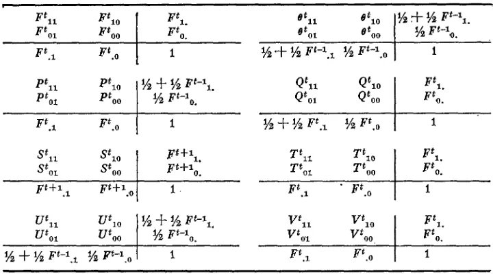
M A R G I N A L TOTALS

The four components of each of the measures may be arranged in two by two tables as shown in Table 2. Consider P t i j for example. Ptl. is the value for terms like Prob [aI a.,]. Now a,, aJ are the same gene half the time and identical with probability one, and are different genes half the time and identical with probability

F;;l.

Thus

Pt,,

= (1 f Fty1)/2. However, P1is the value for terms like b o b [bx = bJ] and thus has the value Ft.l. When we combine Ptij and Qtij

we see that

(P'i. f Q'i.)

2

St,. =

Other values are found similarly.

TRANSITION EQUATIONS

Transition equations are found by straightforward, but sometimes tedious, probability arguments. Using F",l= X i j (ayby, azbz) as an example, we know

(5)

SIB MATING WITH LINKED LOCI

TABLE 2

633

Marginal totals of probability measures

parameter ( h = 0 for free recombination, and h = 1 f o r zero recombination). Hence the three classes of uniting gametes and their probabilities are

(1 - X)Z

4 parental x parental

( 5

1

1 - h2

2

parental x recombinant

(1

-

X)Z

4 recombinant

x

recombinant

For the p X p class, the uniting gametes (ayby,azbz) can take with equal probability one of the four possible values ( aib,,aLbL), (aJbJ,aKbK)

,

( aIb1,aJb,,)

,

( aKbK, aLbL) for which the probabilities of the first two are Ft L l and of the latter two are

e t z l ,

with a n average of

(P,,

+

dt%,,)/2. The p X I class of uniting gametes takes

with equal probabilities one of eight possible values and the probabilities for these values are divided equally between P t , , and QtLl to give an average of

( P t I l

+

Q t 1 3 ) / 2 = St%,. Finally for the I X I class the equally probable four values

have an average probability of

( U t L 3

+

V t L 3 ) / 2 . Multiplying together the probabilities of the classes and the probabilities given the classes leads to the first of the transition equations (6).

(6)

634 C. C . COCKERHAM A N D B. S. WEIR

system. It is only the equation for Stij that necessitates the use of the probability measure Tt;i.

The equations (6) are shown in their simplest possible form by making use of the expressions for the marginal totals as shown in Table 2, and are true for

i

and j taking values 0 or 1. Each equation thus represents four equations. Be- cause of these marginal totals, and the fact that Ft,,, Ft., satisfy equations ( 1 ) ,

it is necessary to solve equations (6) for only one component of each function in order to have solved the whole system. For simplicity we work with the XtoO's.

-

(

F A )

2 ( F A ) 2

0

- -

l,+X) ( l.+A) 1 -A2

8 8

2.

8 8

0 0 0 0

ll+A2

4

0 0

1

7

4

0 0

I - X I - A l + X l + A

- - -

-

1

-

8 I

4

I 8 0 -I

8

a

2

0 0 0 0 0

1

. 8 8

2 l

o

8

I

-

8

- -

-

L L

-

I

-

The six equations for the

XtOO's

may be written in matrix form as in equation (7), ut = Aut_l where A is the transition matrix and U is a vector of six elements.

- -

Foe

e

00

so0

Too

U 0 0

voo

.

--~

Foo

Boo

s o 0

Too

U00

voo

. .

-1

(7)

If the initial members are a pair of outbred, unrelated individuals, the initial 1,+*2 1 1

(7)

SIB MATING WITH LINKED LOCI 635

We now (wish to use (7) to establish a recurrence formula for FtO,, i.e., we want to express Ft,, in terms of only

Foe's

in previous generations. The simplest such equation is, in general, found by way of the minimal polynomial f(s) of the matrix A . This is the simplest polynomial with f ( A ) equal to the zero matrix. Hence f ( A ) ut = 0, and we have a recurrence formula for the whole vector ut,

and so certainly for one component (Foe) of the vector. This ignores the possi- bility of factorization of

f(x)

but, in general, for our matrix A the minimal polynomial has no factors and is equal to the characteristic polynomial and thus

of degree six. The recurrence formula for FtO0 must, therefore, go back six generations, and is now displayed together with the initial six values assuming a non- inbred initial population:

(8) ( 2 + 8 ~ + 6 ~ ~ + 6 ~ ~ + ~ ~ ) t + 3 -

x

( 1 , + 2 ~ + 2 ~ 3 + ~ 4)

Foo 256

-

128

h(1+5X2+2A4) Ft+l - x3 (i+x*)

no 2048

'Ik'

1024

F;o = 1

F;,, = 1

F& =

F&

= (1 004-1 6h2+22X3-t1 7X4+4h5+XG)/256

Fi0 =

(5

124- 1 1 2h2+ 1 2 4 W 1 38A4+76X5+45hG+ 14h7$3X8) /2M8

F;, = ( 2 0 7 4 + 7 0 ~ X 2 + 8 0 0 X 3 + 8 4 8 x 4 f 5 9 2 X 5 ~ 5 3 2 x G f 3 0 6 x 1 1 8+3X2-k2X3+X4

32

32h9+5x10) /16384.

(9)

1

4

Using FiO and FZl = FZl = - leads to

Fql

= (2+3X2+2X3+X4)/32 as given by

I n two special cases, equation (8) reduces considerably. For complete linkage previous authors (

HALDANE

( 1937), SCHNELL ( 1961 ) )

.

( h = l ) the characteristic polynomial of the matrix factorizes to:

(x- % ) ( x u

%)

(Zf % > ( s + $48) ( x 2 -

?h

x-

%),

while for zero linkage (h=O) it factorizes to:

x 3 ( 2

4-

%)

(st' -

%

5 4- 1/16).

In such cases, we take the smallest number of factors (so that the recurrence formula goes back the least number of generations) to form the polynomial g(x)

such that g ( A ) u t has zero first component. By doing so for complete linkage we get equation (10) which is satisfied by FA, and

F",

as we expect for two genes being transmitted as one unit. For zero linkage we get equation (11) which is satisfied by (Fi F t J , which we also expect since now the two genes are transmitted independently.

Ft,, = F;;I

+

F;;'

.

(10)

0 0 00 00 /64 F;i3

.

(11)

(8)

636 C. C. COCKERHAM A N D B. S. WEIR

Of course these two results may be derived without having to go to the sixth degree characteristic equation. For complete linkage, the complete set is just

[Fz,,

8,,lt

and

e,,

may be eliminated easily for all values of

i

and j . For zero

linkage we see that

F t l

= T f l = V t and

O i l

=

U t ,

so that the complete set is [ F 2 , , S,,,

U,,]

t. Here again it is simple, especially for

i

= j = 0, to eliminate

T:,

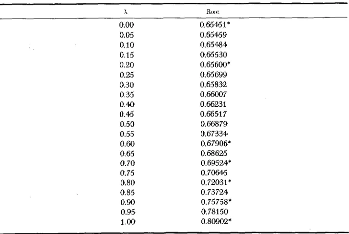
and U:,.

As t increases, the ratio between successive values of F,", tends to the largest

characteristic root of matrix A. When = 1 this value is E = ( 1

+

d 5 ) / 4 as in FISHER (1949)

,

and when = 0 the value is E ~ . Intermediate values are given in

Table 3, where values marked with an asterisk have also been found by BENNETT

(1954).

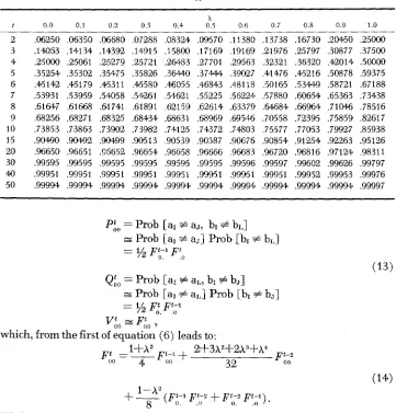
Numerical values of F:, are given in Table 4. Calculations were made for F&

and the one locus inbreeding coefficients assuming that there was no initial inbreeding at either locus, and

Ftll

was computed as follows:

2.1

Ft,,=

Fit,

f F:

4-

Ft,

-

1

.

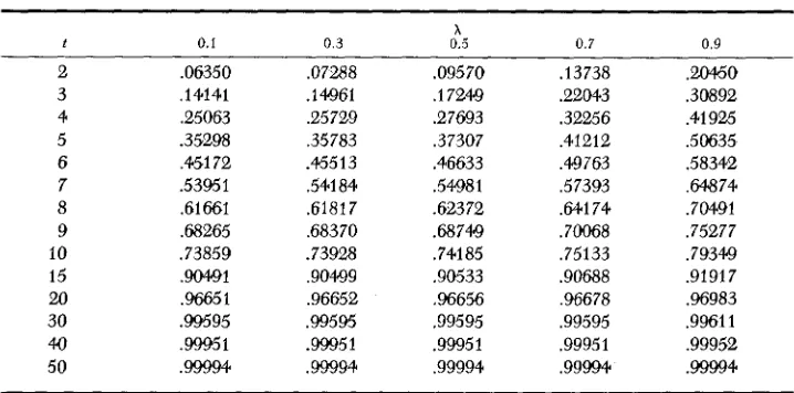
(12)

APPROXIMATION

An approximation can be made which simplifies the recurrence formula considerably, yet yields good numerical results. We replace Pt,;

Q f l

with the values they would have for unlinked loci and replace V:, by

F f , .

Now we are able to write

TABLE 3

Largest characteristic root of transition matrix

~~~

x

Root

0.00 0.65461'

0.05 0.65459

0.10 0.65484

0.15 0.65530

0.20 0.65600*

0.25 0.65699

0.30 0.65832

0.35 0.66007

0.40 0.66231

0.46 0.66517

0.50 0.66879

0.55 0.67334

0.60 0.67906*

0.65 0.68625

0.70 0.69524*

0.75 0.70646

0.80 0.72Q3 1 *

0.85 0.73724

0.90 0.75758*

0.95 0.78 150

(9)

SIB MATING WITH LINKED LOCI

TABLE 4

Numerical values of Ftll f o r selected values of

63 7

1 0.0 0.1 0.2 0 . 3 0.4 0.5 x 0.6 0.7 0.8 0.9 1.0

2

3 4 5 6 7 8 9 10 15 20 30 4.0 50

,06250 ,06350 ,06680 .07288 .08324 ,09570 ,11380 .I3738 .16730 .2WO .25COO ,14053 ,14134 .14392 .I4915 ,15800 ,17169 ,19169 ,21976 ,25797 ,30877 ,37500

.35254 ,35302 ,35475 ,35826 .3WO ,374.1.1. ,39027 ,41476 .45216 ,50878 ,59375 .45142 ,45179 .45311 ,45580 ,46055 ,46843 .48118 ,50165 .53449 ,58721 .67188

,61647 ,61668 .GI741 ,61891 .62159 ,62614 ,63379 .64.684 .66964 ,71046 ,78516

,73853 ,73863 ,73902 .73982 ,74125 ,74372 ,74803 .75.577 ,77053 ,79927 ,85938 .9MO ,90492 ,90499 ,90513 ,90539 ,90587 90676 ,90854 .91254 ,92263 .95126 96650 ,966'51 .96652 .96654 ,96658 ,96666 ,96683 ,96720 93816 ,97124 ,98311 ,99595 .99595 .99595 .99595 ,99595 .99595 .99596 ,99597 ,99602 ,99626 .99797 ,99951 ,99951 ,99951 ,99951 .99951 .99951 .99951 ,99951 .99952 .99953 .99976 99994 ,99994- ,99994 .99994 ,99994 ,99994 ,99994 ,99994 .99994 .99994 .99997 ,25000 .25061 .25,279 ,25721 ,26483 ,27701 ,29563 ,32321 ,36320 .42014 .50000

,53931 .53959 .54058 .54261 .546821 ,55225 ,56224 ,57880 .WO654 ,65363 ,73438

,68256 ,68271 ,68325 ,68434 ,68631 ,68969 .66546 ,70558 .72395 .75859 ,826'17

Pio

= Probs [a,

+

aJ, bI

+

bL]

=

Prob [a,

+

aJ] Prob [bI i bL]

=

1/2

F:;' F f o

Q&

= Probs [a1

+

aL, b l + b ~ ]

=

Prob [aI

+

aL] Prob [bI

P

bJ]

=

%

Fi.

Ftil

Vio s

Fio

,

which, from the first of equation (6) leads to:

While this approximate equation holds exactly for zero or complete linkage, it is also good for intermediate linkage as can be seen by comparing the results in Table 5 with those in Table 4.

DISCUSSION

(10)

638 C. C . COCKERHAM A N D B. S. WEIR

TABLE 5

Approximate values of F,,

x

t 0.1 0 3 0.5 0 7 0.9

2 .06350 ,07288 .09570 .I3738 ,20460

3 ,14141 .I4961 .1 7249 .22043 .30892

4 ,25063 .25 729 .27693 .32256 .41925

5 .35298 ,35783 .37307 ,41212 ,50635

6 ,45172 .45513 .46633 ,49763 .58342

7 .53951 .54184 .5@8 1 ,57393 .&4874 8 ,61661 .61817 .623 72 ,641 74 .70491

9 68265 .68370 5874.9 .70068 .75277

10 .73859 .7392a ,741 85 ,75133 ,79349

15 .!XI491 ,90499 .go533 .go688 .91917

20 .96651 .96652 ,96656 ,96678 .96983

30 99595 ,99595 .99595 ,99595 .99611

40 99951 99951 99951 .99951 .99952

50

.m

.99994 ,99994 .99994 . m 4

modated for any number of loci with just digametic probability measures. For sib mating it was found that two types of trigametic, S and T , and two types of quadrigametic, U and V , probability measures were sufficient, in conjunction with the digametic ones, to provide transitional equations from one generation to the next. Not all types of tri- and quadrigametic probability measures necessary for a general pedigree analysis of two locus inbreeding are encountered in sib mating, however. These are to be developed elsewhere.

Some generalizations are clear at this point. The x-gametic probability measures required for a joint treatment of n linked loci are x = 2,3,

.

. 2 n , but in the analysis of systems of mating x is limited such that x = 2,3,

. . .

2N, where N is the number of individuals. Thus, for selfing and any number of loci, x = 2; for sib mating, x = 2 for n = 1 and x = 2,3,4 for n 2 2; for double first cousins,

x

= 2 for n = 1, x = 2,3,4 for n = 2, x = 2,3,4,5,6 for n = 3 and

x

= 2,3,4,5,6,7,8 for n 2 4; and so on. What is not clear is the number of types required for measures of each order x, as related to the system of mating. I t is the total number of measures which determines the rank of the transitional matrix, e.g., A in (7).

While we do not at this point see how to generalize the rank of A for sib mating and any number of loci, the number of measures for a particular number of loci can be found by the same method demonstrated for two loci.

The set of measures in ( 7 ) is the fewest for transition from one generation to the next. They may be reduced to smaller sets. For example, one may eliminate

8 , T , and

U

to provide a set of three measures but the transition formulae go back three generations. In essence it is the reduction of the set into one measure which leads to the recurrence formula (6) but which goes back six generations.

(11)

SIB MATING WITH LINKED LOCI 639

cified to be identical at either or both loci in either or both initial individuals, and in various ways between individuals. Initial measures must be adjusted accordingly, and different values of the same type of measure are averaged. This points out the fact that averages have been used in two different ways. For example, consider the four F probabilities in Table 1. These are identical to each other regardless of the initial conditions. On the other hand, the two 0’s may be initially different, and if so the arithmetic average is to be used. The same applies to the other measures when they are initially different. If all four genes at one locus of the two initial individuals are identical by descent then all Xloo’s are zero, and inbreeding at the other locus is accounted for by the equations in (6).

It should be stressed that linkage affects only joint probabilities,

F,,,

Flu, F,,

and F,,, of identity by descent of genes, and in no way affects the inbreeding

coefficient,

F ,

or F.,. One must reflect then on the purposes to be served by the joint probabilities, of which two come readily to mind. One has to do with the distribution of multiple zygotes and the other has to do with the variance of “identity by descent” among linked loci ( SCHNELL 1961). Complete information for the variance is provided by two locus probabilities.

To see the effect on the distribution of multiple zygotes, let

atll

= Ftll - F t l , F‘

,

st,,

= Ft,, - Ft,, F‘ 0

atol

=

Pol

- F‘, F f a t o o = Ft,, - Ft,, Ft,o

(15)

,

and note that

at,,

= S t ” , = - a t l o =

-af”,

.

₍₁₆₎

In Table

4

the values under X = 0.0 are equivalent to Ft,. F t . , . By comparing corresponding values for other X’s we see that S1, 2 0, that it increases with h,

that it is maximum for any h in one of the first three generations and that it decreases in time to zero. Thus the effect of linkage is to increase the frequency of double homozygotes over that expected for genes which recombine freely. At the same time, using (16), we note that the frequency of double heterozygotes is affected the same way and that the frequencies of the single heterozygotes are reduced correspondingly. The fact that all 6’s go to zero with time is a reflection of the approach to fixation at both loci.

Similar effects of linkage, but more pronounced, are found

with

selfing

(

NARAIN

1965) where

a t o n = Ft,,

-

Ft,. Ft.,

Suo = SI, being maximum in the first generation.

(12)

640 C. C . COCKERHAM A N D B. S. WEIR

leads to a correlation between genotypes of the two loci, but that the effect is transient and disappears as the individuals become homozygous.

SUMMARY

Sib mating with two linked loci is studied. Trigametic and quadrigametic probability measures of identity by descent are introduced in addition to the usual digametic ones. A minimal set of six measures is required for transition from one generation to the next. When reduced to the panmictic function the recurrence relation goes back six generations. The panmictic function in conjunction with the inbreeding coefficient provides the inbreeding function. Numer- ical values of the inbreeding function, of the largest characteristic root of the transition matrix, and of an approximation to the inbreeding function are given. -Some generalizations concerning the effects of the system of mating and number of loci on the types of probability measures required, concerning the effects of linkage on the inbreeding function and concerning the utility of the inbreeding function are discussed.

LITERATURE CITED

BENNETT, J. H., 1954

F I S H E ~ R. A., 1M9 HALDANE, J. B. S., 1937

The distribution of heterogeneity upon inbreeding. J. Roy. Statist. SOC. B 16: 88-99.

T h o r y of Inbreeding. Oliver and Boyd Ltd., Edinburgh.

Some theoretical results of continued brother-sister mating. J. Genet.

34: 265-274.

-

1949 The association olf characters as a result of inbreeding and linkage. Ann. Eugenics 15: 15-23.

Inbreeding and linkage. Genetics 16: 357-374. HALDANE, J. B. S., and C. H. WADDINGTON, 1931

M A L ~ Y T , G., 1948

NARAIN, P., 1965 Homozygosity in a selfed population with a n arbitrary number of linked loci. J. Genet. 59: 254-266.

SCHNELL, F. W., 1961 Some general formulations of linkage effects in inbreeding. Genetics

46: 947-957.

The generalized inbreeding coefficient in a Markov process. Rep. Statist. Appl. Res., JUSE 9: 127-136.

-

1965a A generalization of the inbreeding coefficient. Biometrics 21: 665-681.

-

196513 Limit of application of generalized inbreeding coefficient and generalized coefficient of parentage. Ann. Repts. Research Group Biophys. Japan 5 : 65-66.

Les MntMmtiques de L'Hiriditk. Masson et Cie., Pans.

SHIKATA, M., 1962