A note on the cost of computing odd degree isogenies

A note on the cost of computing odd degree isogenies

Daniel Cervantes-V´

azquez and Francisco Rodr´ıguez-Henr´ıquez

Computer Science Department, CINVESTAV-IPN

[email protected]

[email protected]

Abstract

Finding an isogenous supersingular elliptic curve of a prescribed odd degree is an important building block for all the isogeny-based protocols proposed to date. In this note we present several strategies for the efficient construction of odd degree isogenies, which outperform previously reported methods when dealing with isogeny degrees in the range [7,220_].

1

Introduction

In the last few years there has been an intense interest in finding efficient formulas for computing odd degree isogenies using different models of elliptic curves. Sev-eral authors have found efficient formulas for computing isogenies using Weierstrass curves [17], Edwards, Twisted Edwards and Huff curves [15], Montgomery curves [5], and more recently, Hessian and twisted Hessian curves [7]. Nonetheless, designers of isogeny-based protocols such as SIDH[11], CSIDH[2, 13] and BSIDH[4], regularly prefer to adopt Montgomery and twisted Edwards curve models for their schemes. This is because it is widely believed that for isogeny-based protocols these two el-liptic curve models provide a much more efficient curve arithmetic.

Let q = pn, where pis a prime number and n a positive integer; and let` be an odd number `= 2s+ 1, withs >1.LetE andE0 be two supersingular elliptic curves defined overFq for which there exists a separable degree-`isogenyφ:E→E0

defined over_Fq.This implies that there must exist an`-order pointP∈E(Fq) such

that Ker(φ) ={∞,±P,±[2]P, . . . ,±[s]P}.Given the domain elliptic curveEand an `-order pointP ∈E(_Fq),in this note we are interested in the problem of computing

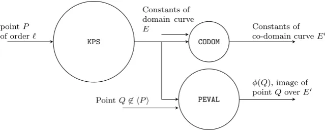
the co-domain elliptic curve E0. Furthermore, given a pointQ ∈ E(_Fq) such that Q6∈Ker(φ),a closely related problem is that of findingφ(Q),i.e., the image of the pointQoverE0.1

In order to find efficient formulations for the above two problems and inspired in the notation used in [10, Table 1], we define KPSas the task of computing the first s multiples of the point P, namely, the set {P,[2]P, . . . ,[s]P}. Using KPS as

1_{We will sometimes refer to these two problems as the isogeny construction and the isogeny evaluation}

KPS CODOM

PEVAL

pointP

of order`

PointQ6∈ hPi

Constants of domain curve

E Constants of

co-domain curveE0

φ(Q),image of pointQoverE0

Figure 1: Given a supersingular elliptic curve

E

and an order-

`

point

P

∈

E

(

F

) this

diagram shows the main modules for computing a degree-

`

isogeneous curve

E

and the

image of a point

Q

∈

E

(

F

)

,

subject to the condition that

Q

is not in the kernel subgroup

6∈ h

P

i. The circles are drawn to scale the relative computational costs of the modules.

a building block, the module CODOM computes the per-field constants that deter-mine the co-domain curveE0 defined over _Fq.Also, usingKPSas a building block,

PEVALcomputes the image pointφ(Q).

Figure 1 shows the dependencies among theKPS,CODOM andPEVAL primitives, where the circles are drawn to scale the relative costs of these three tasks.2_{. Both}

CODOMandPEVALrequire the points in Ker(φ) as input parameters, which are com-puted by theKPSprimitive. Notice that sinceCODOMandPEVALshow no dependen-cies between them, once that the kernel points have been computed, it is possible to computeCODOM and PEVALin parallel. Furthermore, when evaluating an arbitrary number of points inEthat do not belong to the Ker(φ) subgroup,KPSmust be com-puted only once. Hence, the computational cost associated toKPS gets amortized when computing the image of two or more points.

A Montgomery curve [14] is defined by the equationEA,B:By2=x3+Ax2+x,

such thatB 6= 0 andA26= 4.For the sake of simplicity, we will write EA forEA,1.

Moreover, it is customary to represent the constantAin the projective space_P1 _as (A0_:C0_{),such thatA=A}0_/C0 _{(see [6]). In [1] it was shown that every Montgomery}

curve EA,B :By2 =x3+Ax2+xis birationally equivalent to a twisted Edwards

curveEa,d:ax2+y2= 1 +dx2y2. The curve constants are related by

(A, B) =

2(a+d) a−d ,

4 a−d

and (a, d) =

A+ 2

B , A−2

B

.

Table 1 summarizes the field arithmetic costs associated to theKPSandPEVAL op-erations. Note thatKPSis a straightforward computation that can be performed at the cost of one point doubling and k−2 point additions. Efficient formulas for computingPEVALcan be found in [5] and [3] for Montgomery and twisted Edwards curves, respectively.

In the remainder of this note, different strategies for the efficient computation of theCODOM operation will be discussed. A Magma implementation of all the

proce-2

Primitive M S A

Montgomery[5] Edwards[3]

KPS 4(s−1) 2(s−1) 6s−2 6s−2

PEVAL 4s 2 6s 2s+ 4

Table 1: Current State-of-the-art costs for

KPS

and

PEVAL

. Field multiplication (

M

)

and squaring (

S

) costs are taken from [5] and [3]. We are using the fact that

KPS

can

be computed by performing one point doubling and

s

−

2 point additions. The

compu-tational costs associated to the point addition and point doubling operations is of 4

M

+

2

S

+ 6

A

and 4

M

+ 2

S

+ 4

A

, respectively.

dures described here along with theKPS,CODOMandPEVALprimitives, are available at,https://github.com/dcervantesv/Odd_Degree_Isogenies.

2

Twisted Edwards curves

In [15], Moody and Shumov presented `a la V´elu formulas for computing isogenies on Edwards, twisted Edwards and Huff curves. Later, Meyer and Reith in [13] utilized a projective version of those formulas working on twisted Edwards YZ-coordinates. Arguably, these formulas are more efficient than the corresponding to Montgomery curves [5]. In the following, the projective version of Corollary 1 of [15] using Edwards YZ-coordinates will be assumed.

Proposition 1. Let us suppose that F is a subgroup of the twisted Edwards curve Ea,dwith odd order`= 2s+1, s >1.Let the points inF be given in twisted Edwards Y Z-coordinates as the set,

{(Y1:Z1), . . . ,(Ys:Zs)}.

Then, there exists a degree-` isogeny ψ with kernel F that takes us from the curve Ea,d to the curveEa0_,d0. The constantsa0, d0 can be computed as,

By=

s Y

i=1

Yi; Bz= s Y

i=1

Zi; a0=a`B8z; d

0_=B8

yd

`_{. (1)}

Proof. From Corollary 1 of [15], if we consider F0 ={∞,(±α1, β1), . . .(±αs, βs)},

then from the curveEa,d to the curve E¯a,d¯there exists a degree-` isogeny ψ0 with kernelF0 that can be computed as,

B=

s Y

i=1

βi; ¯a=a`; d¯=B8d`. (2)

Usingβi=Yi/Zi and plugging in into Eq. (2) yields,

B= s Y i=1 Yi Zi = Qs i=1Yi Qs

i=1Zi = By

Bz

; ¯a=a`; d¯= (By Bz

)8d`.

It is known from [1] thatEa,d∼=E1,d/a.This implies that

E_¯a,d¯∼=E 1,(

By Bz)8d`

a` ∼

=E 1,B

8

y d` B8

z a` ∼

The computational costs associated to Eq. (1) can be upper bounded by assuming that the exponentiations to the power`are performed independently and by means of the binary method. Let H(`) andλ(`) denote the Hamming weight and the bit-length of the integer `, respectively. Hence, the cost of computing the co-domain curve is given as follows. The valuesB8

y andB8z can be computed at a cost of 2(s−

1)M + 6S. When using the binary method the overall cost of the exponentiations a`<sub>andd</sub>`_{is of 2(H(`)−1)M+ 2(λ(`)−1)S. Two more multiplications are required}

to obtain a0 and d0. Therefore, the cost of computing the constants a0 and d0 of Eq. (1), which define the co-domain isogenous curve is upper bounded by

2(s+ H(`)−1)M + 2(λ(`) + 2)S.

In the remaining of these note, several methods for improving the above upper bound will be discussed.

2.1

Using NAF for reducing the computational cost of odd

degree isogenies

By exploiting once again the property Ea,d ∼= E1,d/a, one can in general reduce

the computation of the exponentiations of Eq. (1) using any signed representation of the exponents such as the well-known Non-adjacent Form (NAF). Let us recall that the NAF representation of a positive integer`is an expression`=Pn_i=0−1`i2i,

where`i∈ {0,±1}, `n−16= 0 and no two consecutive digits `i are nonzero [9]. Let L=N AF(`). In the case of Eq. (5), one can notice that the positive and negative values of the NAF representation of`can be split as,

L=Lp−Lm, where Lp= n−1

X

i=0|ki>0

`i2i, and Lm=− n−1

X

i=0|ki<0

`i2i. (3)

As an illustrative example, let us consider the representations of the integer 353,

(353)2= (1,0,1,1,0,0,0,0,1);

L=N AF(353) = (1,0,¯1,0,¯1,0,0,0,0,1);

(Lp)2= (1,0,0,0,0,0,0,0,0,1);

(Lm)2= (0,0,1,0,1,0,0,0,0,0).

Using the above split NAF representation, one can computen` <sub>asn</sub>Lp<sub>n</sub>−Lm<sub>.</sub> More-over, exploitingEa,d ∼=E1,d/a, one can computea0=a`Bz8andd0 =B8yd` as,

a0=B_z8aLp_dLm_{, d}0 _=B8 ya

Lm_dLp_{. (4)}

We carefully exploit the dependencies on these four exponentiations as shown in Algorithm 1. The accumulators for the exponentiations (aLp_{, a}Lm_{) and (d}Lp_{, d}Lm_), are stored into the two-entry arraysTaandTd,respectively. Notice that in lines 6-7,

these arrays are initialized to one. As we are dealing with odd`, this implies that the least significant bit ofN AF(`) is always non-zero. This observation is used to save two multiplications as shown in line 9. Depending on the sign ofL[0],in line 9 only the entries that will store the positive (or the negative) bit exponentiations get initialized with a and d, respectively. The other entries are only initialized when a sign change is detected. To simplify the algorithm, this change of sign can be pre-computed off-line, by recording the exact position ω where this change occurs. The two input parametersa, dare rewritten to accumulate the squaring operations by updating them at each iteration of the two main loops in lines 10 and 21. They are also updated in line 18 when a sign change has been detected. It can be shown that the cost of computinga0 andd0 using Algorithm 1 is given as,

2(s+ H(L))M + 2(#L+ 2)S,

where L = N AF(`). The above cost is often cheaper than the one presented in the previous section for a binary representation. This is due to the fact that the average non-zero density 1/3 of the NAF representation, is cheaper than the average non-zero density 1/2 of the binary representation.

If the NAF expansion of`contains no ¯1,thenN AF(`) = (`)2and a simple binary exponentiation suffices. In this case the computational expense of Algorithm 1 becomes 2(s+ H(`)−1)M + 2(λ(`) + 2)S. Therefore, it can be concluded that computing an isogeny using Algorithm 1 adds no extra costs, but savings due to the fact that the NAF recoding guarantees a smaller non-zero density in comparison to the binary method.3

As a relevant practical example, consider all the prime factors in the factor-ization of (p512 + 1)/4 where p512 is the prime used in the CSIDH-512 proto-col [2]. The NAF trick discussed here will have the same computational cost as the one associated to the binary representation for those primes in the set

{5,17,37,41,73,137,149,257,277,293,337}. For all the other 63 prime factors of (p512+ 1)/4, the NAF representation produces savings compared with the cost of the binary one. The Magma code of Algorithm 1 is available at,https://github. com/dcervantesv/Odd_Degree_Isogenies.

Remark 1. When Algorithm 1 deals with the case`2 =N AF(`), the variablewL

must be set to any position in the vectorLwith value zero. This way, the assignment on lines 19-20 does not interfere with the positive accumulator as the sign computed in Line 17 is the opposite of the first sign computed (that must be positive as `2 = N AF(L)). On Line 29 if L[ωL] = 0, then a0 and d0 are computed as in

Equation 1. Otherwise,a0 _andd0 _{are computed as in Equation 4.}

Remark 2. We are not aware of any isogeny-based protocol where the input param-eter`of Algorithm 1 must remain secret. Hence, no efforts to protect this procedure against timing-attacks were attempted.

3

Algorithm 1

Odd degree isogenous codomain curve computation using NAF recoding.

Require: Integer`= 2s+ 1, Integer vectorL=N AF(`), IntegerωL∈[0..(#L−1)] in which the first change of

sign occurs. Edwards curve constantsaandd, SubgroupF = (Y1:Z1), . . . ,(Ys:Zs).

Ensure: a0andd0defining the Twisted Edwards curveEa0_,d0 isogenous toEa,das in Corollary 1. 1: By←Y1;

2: Bz←Z1;

3: fori=2tosdo

4: By←ByYi;Bz←BzZi; 5: end for

6: Ta←[1,1]{Initialization ofTa which will holdapandam} 7: Td←[1,1]{Initialization ofTdwhich will holddpanddm} 8: Sign←L[0]+1₂ ;

9: Ta[Sign] =a;Td[Sign] =d; 10: fori:= 1to(ωL−1)do 11: a←a2_;d←d2_;

12: if L[i]6= 0then

13: Ta[Sign]←Ta[Sign]·a; 14: Td[Sign]←Td[Sign]·d; 15: end if

16: end for

17: Sign←(Sign+ 1) mod 2;{The opposite of the Sign ofL[0]}

18: a←a2_;d←d2_;

19: Ta[Sign]←a; 20: Td[Sign]←d;

21: fori:= (ωL+ 1)to(#(L)−1)do 22: a←a2_;d←d2_;

23: if L[i]6= 0then 24: Sign←L[i₂]+1

25: Ta[Sign]←Ta[Sign]·a; 26: Td[Sign]←Td[Sign]·d; 27: end if

28: end for

29: ifL[wL] = 0then 30: a0←B8

z·Ta[1]. 31: d0←B8

y·Td[1]. 32: else

33: a0_←B8

z·Ta[1]·Td[0]. 34: d0←B8

y·Ta[0]·Td[1]. 35: end if

2.2

Using modular arithmetic for reducing the computational

cost of odd degree isogenies

As previously discussed, the computation of Eq. (1) requires two exponentiations to the power`. These computational expenses can be reduced as follows.

Corollary 1. LetEa,d,F and`be given as in Corollary 1. Let us definek=b`/8c,

and r = ` mod 8. Then, from the curve Ea,d to the curve Ea0<sub>,d</sub>0 there exists a degree-` isogenyψ with kernelF,where the constants a0, d0 can be computed as

a0 = (akBz)8ar; d0= (dkBy)8dr; , By= s Y

i=1

Yi; and Bz= s Y

i=1

Zi. (5)

Proof. It follows immediately from Proposition 1 and the property Ea,d ∼=E1,d/a.

At first glance it may appear that compared with Eq. 1, the computational cost of Eq. (5) has been increased by the addition of two extra multiplications and two exponentiations byr. Nevertheless, we will argue in the following that the new formulation of Eq. (5) can save up to 6Scompared with the costs associated to Eq. 1. To this end, let us first analyze the computation ofar _anddr_{. Since we are dealing}

with odd degree isogenies, there are only four possible remainders modulo 8, namely, r= 1,3,5,7. The cheapest case occurs whenr= 1, because we do not incur in any additional multiplication and we trade two exponentiations to the power`in Eq. (1), by two exponentiations to the powerk=bl

8cin Eq. (5). Further, one can compute the other three possible reminders at a cost of only two extra multiplications as shown in Eq. 6.

[a0, d0] =

 



[((ak_B

z)4a)2a, ((dkBy)4d)2d] r= 3

[((akBz)2a)4a, ((dkBy)2d)4d] r= 5

[(akBza)8d, (dkByd)8a] r= 7

(6)

Then, the cost of computinga0andd0as in Corollary 1 and assumingk >0 is given as

2(H(k) +s)M + 2(λ(k) + 2)S ifr= 1

2(H(k) +s+ 1)M + 2(λ(k) + 2)S otherwise. (7)

We dub this method as thediv8approach.

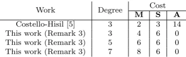
Remark 3. Equation 7 holds for k > 0. When k = 0 one can save one extra multiplication. Therefore, the specialized cost for a degree-3, -5 and -7 isogeny computation using thediv8 approach is of 4M + 6S, 6M + 6S and 8M + 6S, respectively.

2.3

Combining NAF and modular reduction

Corollary 2. Let Ea,d, F and ` = 2d+ 1 as in Corollary 1. Compute K = N AF(bl/8c)and consider

Kp= n−1

X

i=0|Ki>0

ki2i, and Km=− n−1

X

i=0|ki<0

ki2i. (8)

Then, from the curve Ea,d to the curveEa0_,d0 there exists a degree-`isogenyψ with kernelF where

a0= (aKp_dKm_B

z)8ar; d0 = (aKmdKpBy)8dr;

By=

s Y

i=1

Yi; and Bz= s Y

i=1 Zi.

The proof is the same as in Corollary 1 along with a straightforward computation. The cost of computing this new rearrange is given by

2(H(K) +s)M + 2(#K+ 2)S ifr= 1

2(H(K) +s+ 1)M + 2(#K+ 2)S otherwise (9)

The computational cost of the Corollary 2 given in Eq. (9) can be justified as follows,

• Again, in order to computeBy and Bz one requires to perform 2(s−1)M.

• In this case, it is unknown whether the first bit of K is zero or not, but one can pre-compute off-line, how many zeros happen to be before the first non-zero element. Then after initializing the accumulator, one can follow a similar strategy as in Algorithm 1 to computeaKp_{, a}Km_{, d}Kp _{and d}Km_{. This} will help us to save two multiplications. The computational cost of this step is 2(H(K)−2)M + 2(#K−1)S.

• Once we haveBz, By, ar, dr, aKp, aKm, dKpanddKm, the cost of computinga0

andd0 is 6M + 6S.

• Using the result of Eq.(6), it can be seen that two extra multiplications are required to computear _anddr _{forr∈ {3,5,7},and no extra cost for the case} r= 1.

The addition of the above computational expenses gives the result presented in Eq. (9).

3

Comparison

For the sake of fairness, in this section the isogeny construction methods that have been proposed by different authors using their cheapest version for as many odd values` as possible, are reported. Table 2 shows the operation counts for several state-of-the-art isogeny construction algorithms using different elliptic curve mod-els. Note that the a from alpha approach proposed in [5], computes an isogeny construction using the image of a two-torsion point in a Montgomery curve different than the point (0,0). This approach can only be used when considering rational points over an extension of the base field _Fp. Algorithm 3 point recover[5]

Work Model Cost

M S A

a from alpha[5] Mont 4s 4 4s+ 3

3 point recover [5] Mont 8 5 11

CSIDH [2] Mont 6s−2 3 4

Meyer-Reith [13] Ed 2(s+ H(`) 2(λ(`) + 2) 0

Onuki-Takagi [16] Mont 5s−1 2 s+ 5

NAF exp(Algorithm 1) Ed 2(s+ H(L)−1) 2(#L+ 2) 0

div8 r= 1 (§2.2) Ed 2(H(k) +s) 2(λ(k) + 2) 0

div8 r= 3,5,7 (§2.2) Ed 2(H(k) +s+ 1) 2(λ(k) + 2) 0

div8NAFr= 1 (§2.3) Ed 2(H(K) +s) 2(#K+ 2) 0

div8NAFr= 3,5,7 (§2.3) Ed 2(H(K) +s+ 1) 2(#K+ 2) 0

Table 2: General costs for different state-of-the-art isogeny construction algorithms

(dubbed

CODOM

in Fig 1). Notice that the algorithms from [5] require extra input data to

compute the co-domain curve, and might not be useful on the CSIDH framework. Here

`

= 2

s

+ 1,

k

=

b

`/

8c,

r

=

`

mod 8,

L

=

N AF

(

`

) and

K

=

N AF

(

k

).

Work Degree Cost

M S A

Costello-Hisil [5] 3 2 3 14

This work (Remark 3) 3 4 6 0

This work (Remark 3) 5 6 6 0

This work (Remark 3) 7 8 6 0

Table 3: Specialized formulas for certain odd degree isogenies.

cannot be easily extended to a general scenario other than the key generation phase of the SIDH protocol, where primes of the form p= `ea

a ` eb

b f −1 with `i <5 are

used. The rest of the algorithms reported in Table 2 can easily be applied to more generic settings.

We did not consider hybrid cases where curve constants must be translated into another model of curve or to a better representation of the constants. For example, Onuki and Takagi algorithm [16] returns the constant (A : C). The cost of com-puting the constantsA24andC24required for fast Montgomery curve-arithmetic is not taken into account here. Also for the Edwards curves, the computation of the constante=a−dused in [3] to attain faster curve arithmetic is disregarded. Table 3 summarizes the operation counts of optimized formulas for certain specific isogeny degrees. Among all state-of-the-art algorithms, only [5] reports one specialized al-gorithm for a specific isogeny degree. In Remark 3 of this note, concrete isogeny computation formulas for three specific degrees are given.

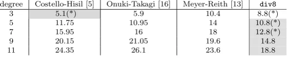
Tables 4 and 5 report the costs of computing the co-domain curve using M as cost metric. In Table 4 it is assumed that S =0.8M as in [16]. For this setting, it is observed that the div8 approach introduced in §2.2 outperforms the other strategies for all the degrees except when computing isogenies of degree 3, where the specialized formula of Costello and Hisil [5] is optimal. Arguably, the assumption of the ratioS =0.8M for the field arithmetic is a bit unrealistic.4 Hence in Table

4_{We still considerS= 0.8Mbecause this might be about the correct ratio for the}

Fp2 quadratic field

degree Costello-Hisil [5] Onuki-Takagi [16] Meyer-Reith [13] div8

3 5.1(*) 5.9 10.4 8.8(*)

5 11.75 10.95 14 10.8(*)

7 15.95 16 18 12.8(*)

9 20.15 21.05 19.6 14.8

11 24.35 26.1 23.6 18.8

Table 4: Costs assuming

S

= 0.8

M

and

A

= 0.05

M

. All costs are given Using

M

as

unit of measure. Costs with(*) indicate that we are using the operation counts reported

in Table 3. The shaded cells indicate the minimum cost for each degree.

degree Costello-Hisil[5] Onuki-Takagi[16] Meyer-Reith [13] div8

3 5.7(*) 6.300 12 10(*)

5 12.55 11.35 16 12(*)

7 16.75 16.40 20 14(*)

9 20.95 21.45 22 16

11 25.15 26.50 26 20

Table 5: Costs assuming

S

=

M

and

A

= 0.05

M

. All costs are given Using

M

as unit

of measure. Costs with (*) indicate that we are using the operation counts reported in

Table 3. The shaded cells indicate the minimum cost for each degree.

5 a more realistic scenario for_Fp arithmetic is considered by assumingS=M . In

this setting the algorithm by Onuki and Takagi [16] emerges as the optimal method when constructing degree-5 isogenies. In the case of degree-3 isogeny constructions, the approach by Costello and Hisil [5] remains unbeatable.

We executed our Magma scripts for determining the associated computational costs for div8, NAFexp anddiv8NAF . We also report the computational costs for Onuki and Takagi [16] and Meyer-Reith [12] analyzed trough all the prime numbers in the interval [11,220]. The corresponding computational costs are summarized in Tables 6 and 7.

The large interval considered in Tables 6 and 7 can be of interest for the search of more conservative parameters for the CSIDH protocol. Moreover, BSIDH[4] uses` -isogenies where the biggest bit-length of`is of about 22 bits. Furthermore, recently the S ´ETA protocol, a new isogeny-based protocol, was introduced in [8]. The S ´ETA protocol seems to make use of`-isogenies where the largest`is about 214_.

Remark 4. We only consider odd prime degree isogenies due to the following obser-vation. Let us assume that one wants to compute a composite odd degree-`isogeny with ` = Qr_i=1`i, `i being distinct prime numbers and r > 1 a positive integer.

Such isogeny can be computed as the composition of therdegree-`iisogenies. It is

not hard to see that using that composition approach, the associated computational complexity is linear5 _{with respect to} Pr

i=1`i. If one would try to compute the `

-degree isogeny by directly applying the formulas presented in this document, the computational complexity is also linear but this time with respect toQr_i=1`i.The

latter is a much larger number than the one associated to the composition approach.

5_{And possibly linear-logarithmic with respect to} Qr

Vs. Meyer-Reith [13] Onuki-Takagi [16] NAFexp div8 div8NAF

Meyer-Reith [13] - 100 6.163 0 0

Onuki-Takagi [16] 0 - 0.001 0 0

NAFexp 77.649 99.998 - 24.004 0

div8 100 100 62.254 - 9.408

div8NAF 100 100 100 67.239

-Table 6: Comparison of different algorithms to compute

CODOM

, assuming

S

=

M

and

`

6=

N AF

(

`

) for a prime

`

∈

[11

,

2

]. All numbers report the winning percentage when

comparing the algorithm in row

i

versus the algorithm in column

j

. Since for some

degrees there are ties, it may occur that the addition of the cells (

i, j

) + (

j, i

) could be

smaller than 100.

Vs. Meyer-Reith [13] Onuki-Takagi [16] NAFexp div8 div8NAF

Meyer-Reith [13] - 100 6.163 0 0

Onuki-Takagi [16] 0 - 0 0 0

NAFexp 87.379 100 - 37.745 0

div8 100 100 62.254 - 9.408

div8NAF 100 100 100 79.884

-Table 7: Comparison of different algorithms to compute

CODOM

assuming

S

= 0.8

M

and

`

6=

N AF

(

`

) for a prime

`

∈

[11

,

2

]. All numbers report the winning percentage when

compare the algorithm in row

i

versus the algorithm in column

j

. Since for some degrees

there are ties, it may occur that the addition of the cells (

i, j

) + (

j, i

) could be smaller

than 100.

4

Conclusion

The cost of constructing odd-degree isogenies on Edwards curves is closely related to the problem of the simultaneous computation of several exponentiations over_Fq.

In this note we review three strategies to compute such exponentiations. Our results show that for most prime numbers in the interval [11,220_{] the div8NAF approach} described in this note appears to be the best option for computing odd degree isogenies on Edwards curves. On the other hand, if we focus on the prime numbers that appear in the factorization of the prime p512+ 1 used in [2], it seems that thediv8 approach is the best (See Appendix A). Moreover, for the relevant case of isogenies of degree 3, the best algorithm is the one provided by Costello and Hissil in [5]. The best approach for constructing degree-5 isogenies is contested between ourdiv8 approach and the Onuki and Takagi [16] algorithm. The former strategy is better when it is assumed thatS=0.8M, but the latter is cheaper whenS=M. The main contribution of this note is the introduction of the NAF exponentiation into the Edwards co-domain curve computation (§2.1) and the div8 (§2.2) and

Acknowledgements

This work was done while the authors were visiting the University of Waterloo. The authors would like to thank Jos´e Eduardo Ochoa-Jim´enez for his useful comments.

References

[1] Daniel J. Bernstein, Peter Birkner, Marc Joye, Tanja Lange, and Christiane Pe-ters. Twisted edwards curves. In Serge Vaudenay, editor, Progress in Cryptol-ogy – AFRICACRYPT 2008, pages 389–405, Berlin, Heidelberg, 2008. Springer Berlin Heidelberg.

[2] Wouter Castryck, Tanja Lange, Chloe Martindale, Lorenz Panny, and Joost Renes. CSIDH: an efficient post-quantum commutative group action. In Ad-vances in Cryptology - ASIACRYPT 2018 - 24th International Conference on the Theory and Application of Cryptology and Information Security, Brisbane, QLD, Australia, December 2-6, 2018, Proceedings, Part III, pages 395–427, 2018.

[3] Daniel Cervantes-V´azquez, Mathilde Chenu, Jes´us-Javier Chi-Dom´ınguez, Luca De Feo, Francisco Rodr´ıguez-Henr´ıquez, and Benjamin Smith. Stronger and faster side-channel protections for csidh. In Peter Schwabe and Nicolas Th´eriault, editors, Progress in Cryptology – LATINCRYPT 2019, pages 173– 193, Cham, 2019. Springer International Publishing.

[4] Craig Costello. B-sidh: supersingular isogeny diffie-hellman using twisted tor-sion. Cryptology ePrint Archive, Report 2019/1145, 2019. https://eprint. iacr.org/2019/1145.

[5] Craig Costello and Huseyin Hisil. A simple and compact algorithm for sidh with arbitrary degree isogenies. Cryptology ePrint Archive, Report 2017/504, 2017. https://eprint.iacr.org/2017/504.

[6] Craig Costello, Patrick Longa, and Michael Naehrig. Efficient algorithms for supersingular isogeny Diffie–Hellman. In Advances in Cryptology - CRYPTO 2016 - 36th Annual International Cryptology Conference, Santa Barbara, CA, USA, August 14-18, 2016, Proceedings, Part I, pages 572–601, 2016.

[7] Thinh Dang and Dustin Moody. Twisted hessian isogenies. Cryptology ePrint Archive, Report 2019/1003, 2019. https://eprint.iacr.org/2019/1003. [8] Cyprien Delpech de Saint Guilhem, P´eter Kutas, Christophe Petit, and Javier

Silva. S ´Eta: Supersingular encryption from torsion attacks. Cryptology ePrint Archive, Report 2019/1291, 2019. https://eprint.iacr.org/2019/1291. [9] D. Hankerson, A. J. Menezes, and S. Vanstone. Guide to Elliptic Curve

Cryp-tography. Springer-Verlag, Secaucus, NJ, USA, 2003.

[10] Aaron Hutchinson, Jason LeGrow, Brian Koziel, and Reza Azarderakhsh. Fur-ther optimizations of csidh: A systematic approach to efficient strategies, per-mutations, and bound vectors. Cryptology ePrint Archive, Report 2019/1121, 2019. https://eprint.iacr.org/2019/1121.

[12] Michael Meyer, Fabio Campos, and Steffen Reith. On lions and elligators: An efficient constant-time implementation of CSIDH. In Post-Quantum Cryptog-raphy - 10th International Workshop, PQCrypto 2019, 2019.

[13] Michael Meyer and Steffen Reith. A faster way to the CSIDH. InProgress in Cryptology - INDOCRYPT 2018 - 19th International Conference on Cryptology in India, New Delhi, India, December 9-12, 2018, Proceedings, pages 137–152, 2018.

[14] Peter L. Montgomery. Speeding the Pollard and elliptic curve methods of factorization. Mathematics of Computation, 48:243–234, 1987.

[15] Dustin Moody and Daniel Shumow. Analogues of velu’s formulas for isoge-nies on alternate models of elliptic curves. Cryptology ePrint Archive, Report 2011/430, 2011. https://eprint.iacr.org/2011/430.

[16] Hiroshi Onuki and Tsuyoshi Takagi. On collisions related to an ideal class of order 3 in csidh. Cryptology ePrint Archive, Report 2019/1209, 2019. https: //eprint.iacr.org/2019/1209.

[17] Jacques V´elu. Isog´enies entre courbes elliptiques. C. R. Acad. Sci. Paris S´er. A-B, 273:A238–A241, 1971.

Appendix A

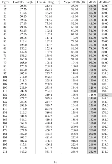
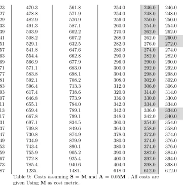
For completeness, we include two Tables with the cost of the other 70 primes on the factorization ofp512+ 1 not included in Tables 4 and 5. We report both cases, when

S= 0.8MandS=M.

Degree Costello-Hisil[5] Onuki-Takagi [16] Meyer-Reith [13] div8 div8NAF

13 28.55 31.15 25.60 20.80 20.80

17 36.95 41.25 29.20 24.40 24.40

19 41.15 46.30 33.20 28.40 28.40

23 49.55 56.40 39.20 32.40 32.40

29 62.15 71.55 45.20 40.40 42.00

31 66.35 76.60 49.20 42.40 44.00

37 78.95 91.75 52.80 48.00 48.00

41 87.35 101.9 56.80 52.00 52.00

43 91.55 106.9 60.80 56.00 56.00

47 99.95 117.0 66.80 60.00 60.00

53 112.6 132.1 70.80 66.00 67.60

59 125.2 147.3 78.80 74.00 73.60

61 129.4 152.3 80.80 76.00 75.60

67 142.0 167.5 84.40 79.60 79.60

71 150.4 177.6 90.40 83.60 83.60

73 154.5 182.6 90.40 85.60 85.60

79 167.2 197.8 100.4 93.60 93.60

83 175.5 207.9 102.4 97.60 97.60

89 188.2 223.0 108.4 103.6 105.2

97 205.0 243.2 114.4 109.6 111.2

101 213.4 253.3 120.4 115.6 117.2

107 226.0 268.5 128.4 123.6 125.2

109 230.2 273.5 130.4 125.6 127.2

113 238.5 283.7 132.4 127.6 127.2

127 267.9 319.0 152.4 145.6 143.2

131 276.3 329.1 150.0 145.2 145.2

137 288.9 344.2 156.0 151.2 151.2

139 293.1 349.3 160.0 155.2 155.2

149 314.1 374.5 170.0 165.2 165.2

151 318.3 379.6 174.0 167.2 167.2

157 330.9 394.8 180.0 175.2 175.2

163 343.5 409.9 184.0 179.2 179.2

167 351.9 420.0 190.0 183.2 183.2

173 364.5 435.2 196.0 191.2 191.2

179 377.1 450.3 202.0 197.2 198.8

181 381.3 455.3 204.0 199.2 200.8

191 402.3 480.6 218.0 211.2 210.8

193 406.5 485.7 212.0 207.2 208.8

197 414.9 495.8 218.0 213.2 214.8

199 419.1 500.8 222.0 215.2 216.8

211 444.3 531.1 234.0 229.2 230.8

223 469.5 561.4 250.0 243.2 242.8

227 477.9 571.5 250.0 245.2 244.8

229 482.1 576.6 252.0 247.2 246.8

233 490.5 586.7 256.0 251.2 250.8

239 503.1 601.8 266.0 259.2 258.8

241 507.3 606.9 264.0 259.2 256.8

251 528.3 632.1 278.0 273.2 268.8

257 540.9 647.2 275.6 270.8 270.8

263 553.6 662.4 285.6 278.8 278.8

269 566.1 677.6 291.6 286.8 286.8

271 570.3 682.6 295.6 288.8 288.8

277 582.9 697.8 299.6 294.8 294.8

281 591.3 707.9 303.6 298.8 298.8

283 595.6 712.9 307.6 302.8 302.8

293 616.6 738.2 315.6 310.8 310.8

307 645.9 773.5 331.6 326.8 326.8

311 654.3 783.6 337.6 330.8 330.8

313 658.6 788.7 337.6 332.8 330.8

317 666.9 798.8 343.6 338.8 336.8

331 696.3 834.1 355.6 350.8 350.8

337 708.9 849.2 359.6 354.8 354.8

347 729.9 874.5 373.6 368.8 370.4

349 734.1 879.6 375.6 370.8 372.4

353 742.6 889.7 375.6 370.8 372.4

359 755.1 904.8 385.6 378.8 380.4

367 771.9 925.0 395.6 388.8 390.4

373 784.6 940.2 399.6 394.8 394.4

Table 8: Costs assumingS= 0.8MandA= 0.05M. All costs are given UsingMas cost metric. Entries with (*) indicate cost using NAF exponentiation.

Degree Costello-Hisil[5] Onuki-Takagi [16] Meyer-Reith [13] div8 div8NAF

13 29.35 31.55 28.00 22.00 22.00

17 37.75 41.65 32.00 26.00 26.00

19 41.95 46.70 36.00 30.00 30.00

23 50.35 56.80 42.00 34.00 34.00

29 62.95 71.95 48.00 42.00 44.00

31 67.15 77.00 52.00 44.00 46.00

37 79.75 92.15 56.00 50.00 50.00

41 88.15 102.2 60.00 54.00 54.00

43 92.35 107.3 64.00 58.00 58.00

47 100.8 117.4 70.00 62.00 62.00

53 113.4 132.5 74.00 68.00 70.00

59 126.0 147.7 82.00 76.00 76.00

61 130.2 152.8 84.00 78.00 78.00

67 142.8 167.9 88.00 82.00 82.00

71 151.2 178.0 94.00 86.00 86.00

73 155.3 183.0 94.00 88.00 88.00

79 168.0 198.2 104.0 96.00 96.00

83 176.3 208.3 106.0 100.0 100.0

89 189.0 223.5 112.0 106.0 108.0

97 205.8 243.7 118.0 112.0 114.0

101 214.2 253.8 124.0 118.0 120.0

103 218.3 258.8 128.0 120.0 122.0

107 226.8 268.9 132.0 126.0 128.0

109 231.0 273.9 134.0 128.0 130.0

113 239.3 284.1 136.0 130.0 130.0

127 268.8 319.4 156.0 148.0 146.0

131 277.2 329.5 154.0 148.0 148.0

137 289.8 344.7 160.0 154.0 154.0

139 293.9 349.7 164.0 158.0 158.0

149 314.9 374.9 174.0 168.0 168.0

151 319.2 380.0 178.0 170.0 170.0

157 331.8 395.2 184.0 178.0 178.0

163 344.3 410.3 188.0 182.0 182.0

167 352.8 420.4 194.0 186.0 186.0

173 365.3 435.6 200.0 194.0 194.0

179 377.9 450.7 206.0 200.0 202.0

181 382.2 455.8 208.0 202.0 204.0

191 403.2 481.0 222.0 214.0 214.0

193 407.3 486.1 216.0 210.0 212.0

197 415.8 496.2 222.0 216.0 218.0

199 419.9 501.2 226.0 218.0 220.0

223 470.3 561.8 254.0 246.0 246.0

227 478.8 571.9 254.0 248.0 248.0

229 482.9 576.9 256.0 250.0 250.0

233 491.3 587.1 260.0 254.0 254.0

239 503.9 602.2 270.0 262.0 262.0

241 508.2 607.2 268.0 262.0 260.0

251 529.1 632.5 282.0 276.0 272.0

257 541.8 647.6 280.0 274.0 274.0

263 554.4 662.8 290.0 282.0 282.0

269 566.9 677.9 296.0 290.0 290.0

271 571.1 683.0 300.0 292.0 292.0

277 583.8 698.1 304.0 298.0 298.0

281 592.1 708.2 308.0 302.0 302.0

283 596.4 713.3 312.0 306.0 306.0

293 617.4 738.6 320.0 314.0 314.0

307 646.8 773.9 336.0 330.0 330.0

311 655.1 784.0 342.0 334.0 334.0

313 659.4 789.1 342.0 336.0 334.0

317 667.8 799.1 348.0 342.0 340.0

331 697.1 834.5 360.0 354.0 354.0

337 709.8 849.6 364.0 358.0 358.0

347 730.8 874.9 378.0 372.0 374.0

349 734.9 879.9 380.0 374.0 376.0

353 743.4 890.1 380.0 374.0 376.0

359 755.9 905.2 390.0 382.0 384.0

367 772.8 925.4 400.0 392.0 394.0

373 785.4 940.6 404.0 398.0 398.0

587 1235. 1481. 618.0 612.0 612.0