Copper Price Prediction Using Support Vector Regression Technique

Article

Copper Price Prediction Using Support Vector

Regression Technique

Gabriel Astudillo1,2 , Raúl Carrasco3,* , Christian Fernández-Campusano4,5 and

Máx Chacón2

1 _{Escuela de Ingeniería Informática, Universidad de Valparaíso, Valparaíso 2362807, Chile}

(e-mail: [email protected])

2 _{Departamento de Ingeniería Informática, Universidad de Santiago de Chile, Santiago 9170124, Chile}

(e-mail: [email protected])

3 _{Facultad de Ingeniería, Ciencia y Tecnología, Universidad Bernardo O’Higgins, Santiago 8370993, Chile}

(e-mail: [email protected])

4 _{Departamento de Ingenierías Multidisciplinares, Universidad de Santiago de Chile, Santiago, Chile}

(e-mail: [email protected])

5 _{University of the Basque Country UPV/EHU, Department of Architecture and Computer Technology,}

Donostia-San Sebastián, Spain

* Correspondence: [email protected] (G.A.) and [email protected] (R.C.)

Received: date; Accepted: date; Published: date

Abstract: Predicting copper price is essential for making decisions that can affect companies and

governments dependent on the copper mining industry. Copper prices follow a time series that is non-linear, non-stationary, and which have periods that change as a result of potential growth, cyclical fluctuation and errors. Sometimes the trend and cyclical components together are referred to as a trend-cycle. In order to make predictions, it is necessary to consider the different characteristics of trend-cycle. In this paper, we study a copper price prediction method using Support Vector Regression. This work explores the potential of the Support Vector Regression with external recurrences to make predictions at 5, 10, 15, 20 and 30 days into the future in the copper closing price at the London Metal Exchanges. The best model for each forecast interval is performed using a grid search and balanced cross-validation. In experiments on real data-sets, our results obtained indicate that the parameters (C,

ε,γ) of the model Support Vector Regression do not differ between the different prediction intervals.

Additionally, the amount of preceding values used to make the estimates does not vary according to the predicted interval. Results show that the support vector regression model has a lower prediction error and is more robust. Our results show that the presented model is able to predict copper price volatilities near reality, being the RMSE equal or less than the 2.2% for prediction periods of 5 and 10 days.

Keywords:Copper price; prediction; support vector regression.

1. Introduction

Copper is one of the first metal products to be listed on the world’s main foreign exchange markets: The London Metal Exchange (LME), Commodity Exchange Market of New York (COMEX) and Shanghai Futures Exchange (SHFE). Copper price is determined by the supply and demand dynamics on the metal exchanges, especially the London Metal Exchange. Although it may be strongly influenced by the currency exchange rate and the investment flow, the factors that can cause fluctuations in volatile prices are partially associated with changes in the activity of the economic cycle [1].

There are many reasons for wanting to make predictions about the price of copper. On the one hand, copper among other natural elements (e.g. silver) has a high electrical and thermal conductivity.

Appl. Sci.2019,xx, 5; doi:10.3390/appxx010005 www.mdpi.com/journal/applsci

On the other hand, it is cheaper than silver and more resistant to corrosion. Therefore, copper is the preferred metal option for electrical and electronic applications, both domestically and for more general industrial uses. Given the importance of the construction and telecommunications sectors in a modern economy, the changes in copper price can be perceived as an early indicator of global economic performance and have a significant impact factor on the performance of related companies [2].

With regard to the copper market, any variation in its demand translates entirely into price fluctuations. Market participants see it as an early sign of changes in global production. Thus, it affects mining companies in their investment plans, traders, investors, agents involved in the copper mining business, and governments dependent on the copper mining industry. To illustrate this, we can consider the particular case of Chile. As the world’s leading copper producer and exporter, Chile produced an estimated 5.6 million metric tons of copper in 2019 [3]. The Chilean government made copper the main point of reference for the country’s structural budget rule introduced in 2000, trying to reduce the exposure of fluctuations in Chile’s GDP to the oscillation of the price of copper [4].

Several studies include copper and other metals as one of the products of interest in the evaluations of the prediction to improve the forecasts of price. Such studies employ different methods and mathematical models such as ARIMA models combined with wavelets [5], meta-heuristics models [6] and neural networks models [2,7,8]. On the other hand, The Fourier Transform [9] is used to analyze the variability of the prices of various metals. In addition, there are works in the literature that study the relationship of commodity and asset price models, such as the case of oil prices and their effect on copper and silver prices. [10–12].

This study applies a copper price prediction method using Support Vector Regression. This work explores the potential of the Support Vector Regression with external recurrences to make predictions at 5, 10, 15, 20 and 30 days into the future in the copper closing price at the London Metal Exchanges. The best model for each forecast interval is performed using a grid search and balanced cross-validation.

2. Previously

In the general case of the financial time series, the methods of Support Vector Machine (SVM) and Support Vector Regression (SVR) are widely used for making forecasts [13]. Basically, when the support vector machine method extends to non-linear regression problems, it is called Support Vector Regression [14–16]. The Support Vector Regression method belonging to the field of data statistics was firstly proposed by Vapnik et al. [14] at the end of the twentieth century. A characteristic of this method is that it solves the problems of “high dimensionality” and “overlearning” to a certain degree. Furthermore, it achieves a significant effect in solving the problem of small samples. Consequently, Support Vector Regression is used to solve the prediction problems of non-linear data in engineering areas.

It is important to consider some works, such as the work done by Kim [17], which presents daily forecasts (by using SVR) of the trend of change in the Korean Composite Stock Price Index (KOSPI), in which it uses 2928 days of data, between January 1989 and December 1998. In another work, Kao et al. [18] use SVR to predict the stock index of the São Paulo State Stock Exchange (Bovespa), the China Composite SSE Index (SSEC) and the Dow Jones, using data from April 2006 to April 2010. Similarly, Kazem et al. [19] predict the market prices of Microsoft, Intel and the National Bank shares, using a set of data from November 2007 to November 2011. In these Works, the prediction is always a day before and depends on a certain amount of past data,l. If ˆpt+1is the price foretold int+1, it has that

ˆ

pt+1= f(pt,pt−1, . . . ,pt−l).

indicates the price change rate and the average data rate, among others. The author uses historical data from January 2003 to December 2012 of the CNX Nifty stock index and S&P BSE Sensex.

3. Support Vector Regression Model

Given a data set ofNelements{(Xi,yi)}Ni=1, whereXiis thei-th element in a space ofndimensions, Xi = [x1,i, . . . ,xn,i]∈ Rn, andyi(yi ∈ R) is the actual value forXi, a non-linear function is defined as

φ:Rn → Rnh_{. To map the entry data,Xiis anR}nh _{space of high dimension called space of features,}

that determines the non-linear transformationφ. So, in a high-dimensional space, there exists a linear

functionf that makes it possible to relate the entry dataXiand outputyi. That linear function, named SVR function, is presented in the Eq.(1),

f(X) =WT·φ(X) +b (1)

where f(X)represents the foretold values;W ∈ Rn_{andb∈ R. The SVR minimizes the empiric risk,} shown in the Eq. (2)

Rreg(f) =C N

∑

Θε(yi−f(Xi)) + 1 2

W

T

(2)

whereΘε(yi−f(Xi))is a cost function. In the case of theε-SVR, a loss functionε-insensitive is used

[14,21], defined in the Eq. (3),

Θε(y− f(X)) =

(

|y−f(X)| −ε If |y−f(X)|>ε

0 In another case (3)

Θεis used to determine the no-linear functionφin theRnh space to find a function that can fit current training data with a deviation less than or equal toε(see Fig.1a). This function minimizes the

training error between the data-training and the functionε-insensitive is provided by Eq. (4) [15,22].

min W,b,ξ∗,ξ

Rreg(W,ξ∗,ξ) = 1

2W

T_W+C

∑

(ξ∗_i +ξi) (4)

subject to restrictions (for all,i=1, . . . ,N):

Yi−WTφ(Xi)−b6ε+ξ∗_i −Yi−WTφ(Xi) +b6ε+ξi

ξ∗_i >0 (5)

ξi>0

The Eq. (4) punishes the training errors of f(X)andYthrough the functionε-insensitive (Fig.1b).

The parameterCdetermines the compromise between the complexity of the model, expressed by the vectorWand the points that fulfil the condition|f(X)−y|>εin the Eq. (3). IfC→∞, the model has

a small margin and is adjusted to the data. IfC→0, the model has a big margin, which is why it is softened. Finally,ξ_i∗represents the training errors greater thanεandξithe errors less than−ε(see Fig. 1a).

To solve this regression problem, we can replace the internal product of the Eq. (1) by functions of KernelK(). This makes it possible to perform such an operation in a superior dimension, using low-dimensional space data input without knowing the transformationφ[23], as it is shown in Eq. (6).

X Y

(a) (b)

Figure 1.Schematic diagram; (a) SVR, and (b) SVR using anε-insensitive function.

f(X) =

N

∑

(β∗−β)·K(Xi,X) +b (6)

The parameters β∗ andβare Lagrange multipliers associated with the problem of quadratic

optimization. Several types of functions can be used as Kernel [24], but in this work, we will be using the Gaussian function of a radial base (RBF)[25]:

K(Xi,X) =exp(−γ||Xi−X||2) (7)

The parametersγof the kernel function, the regularization constantCandεof the loss function

are considered the parameters of design of the SVR to use. Furthermore, they are obtained from a data set that is different from the training data.

4. Data

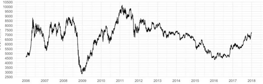
There are three major stock exchanges where the copper is traded: LME, COMEX and SHFE. In this work, we use the closing price of copper given by LME, which is widely considered as a reference index for world prices of this metal[26]. The time series has 2971 data from January 2, 2006 until January 2, 2018, as shown in Fig.2.

One of the parameters of the SVR to be used isε, which has a relation with the tolerance margin of

the punishment of the errors in the training. To choose an adequate range for the subsequent adjustment of parameters, it is necessary to know the level of noiseRthat the time series has. It has an average R=3.66·10−4, a standard deviationSDR=0.068, a medium quadratic errorMSER=0.004624 and a range between[−0.246, 0.205]. This last characteristic allows us to define a conservative Rank for

ε= [0, 0.3].

Figure 2.Evolution of time series of the closing copper price in LME, from January 2006 to January

5. Methodology

In the case of the prediction of time series with SVR, it is assumed that the actual valueytis a function of its previousLvalues~xt= [yt−1, . . . ,yt−L]and the hyper-parameter of the SVR~w= [C,ε,γ].

Hence, the model has four parameters (see Table1); whereLis the number of prior values to predict the actual value and three hyper-parameter of the SVR.

Table 1.Ranges for the grid of the parametersL,C,εandγfor the radial and linear kernel.

Parameter Range

L 1, 2, . . . , 10

C 2−8_{, 2}−7_{, . . . , 2}12 ε 0.01, 0.02, . . . , 0.30 γ 2−8, 2−7, . . . , 212

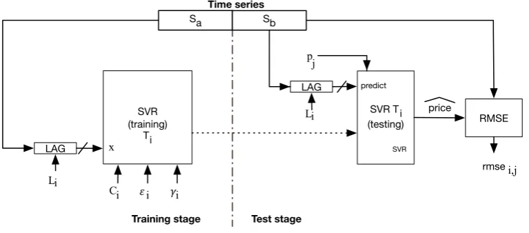
The Rank of each one is shown in Table1. The set of parametersQi={Li,Ci,εi,γi}defines the SVR of trainingi-th (Ti) of the Fig.3. To adjust the parameters and the respective training, the data is normalized in the rank[0, 1]and it is made into a grid search, according to the recommendation of Hsu et al. [27].

The process of training/testing is made using the balanced cross-validation method proposed by McCarthy [28] and shown in Fig.3.

Training stage

SVR (training)

LAG x

(testing)

predict

LAG

RMSE price

rmse

Ci !_i "_i

i,j

SVR

Li

Test stage

Sa Sb

Li p j

Time series

Ti

SVR T i

Figure 3.Training method and adjust the parameters based on balanced cross-validation method.

The series of Fig.2is divided into two series,SaandSb, each one with 50% of the data. First, the SVRTiis trained with one of these two series, with a set of parametersQi. Then, it proceeds to try the capacity to predict with the other half, determining its performance to predictpjdays to future with pj∈ {5, 10, . . . , 30}. The performance will be measured based on the Medium quadratic Error (MSE) between the predicted and the original data.

To make the prediction atpjdays, the SVRTitakes a vector ofLipast values, taking into account the previous predicted values if they correspond with ˆyt+pjas the value to predict in pjdays and~xt+pj

being the vector that contains the previousLivalues that are used in the prediction. Then, you have ˆ

~xt+p_j =[yˆt+(pj−1), ˆyt+(pj−2), . . . , ˆyt+1

| {z }

pj>1

;

yt,yt−1, . . . ,yt−(L_i−p_j)

| {z }

L_i>p_j

] (8)

For the implementation of the training and adjustment system of Fig.3, R, version 3.4.4 was used with the librarye1071[29] for the basic training functions and the librarydoParallel[30] for parallelizing the search of parameters.

6. Results and Analysis

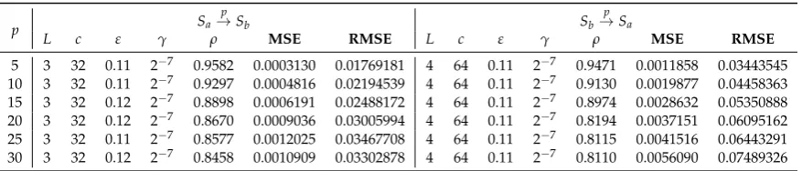
In the experiments, the best models were explored in a grid choosing the best (MSE minor) for eachpprediction interval. Table2shows the parameters for the best SVR, according to the MSE index, for each of training and test and prediction interval ofp. Additionally, it is shown the correlation index

ρbetween the real data and the predicted data and the Root Mean Square Error (RMSE). In Table2,

R→p T means that to train the SVR, the set R∈(Sa,Sb)is used and it is tested in the set T∈(Sa,Sb), with R6=T, wherepis the prediction interval, withp∈(5, 10, 15, 20, 25, 30).

Table 2. Values of the parameters for the best models for each prediction interval according to the

training set and test.

p Sa

p

→Sb Sb

p

→Sa

L c ε γ ρ MSE RMSE L c ε γ ρ MSE RMSE

5 3 32 0.11 2−7 0.9582 0.0003130 0.01769181 4 64 0.11 2−7 0.9471 0.0011858 0.03443545 10 3 32 0.11 2−7 0.9297 0.0004816 0.02194539 4 64 0.11 2−7 0.9130 0.0019877 0.04458363 15 3 32 0.12 2−7 _{0.8898 0.0006191 0.02488172 4 64 0.11 2}−7 _{0.8974 0.0028632 0.05350888} 20 3 32 0.12 2−7 _{0.8670 0.0009036 0.03005994 4 64 0.11 2}−7 _{0.8194 0.0037151 0.06095162} 25 3 32 0.11 2−7 _{0.8577 0.0012025 0.03467708 4 64 0.11 2}−7 _{0.8115 0.0041516 0.06443291} 30 3 32 0.12 2−7 0.8458 0.0010909 0.03302878 4 64 0.11 2−7 0.8110 0.0056090 0.07489326

The best prediction capacity is obtained during the training with the seriesSa, which is temporarily the oldest. The training could have been enhanced due to the level of noise of this series,MSESa =

0.007225, which is higher than the one of the seriesSb,MSESb =0.001024.

It is interesting to note that the amount of previous data (L) is independent of the prediction interval that is made, as well as the parameters of the SVR that remain practically intact. The adjustment capacity for the 5-day prediction of theSa → Sbtime series for the 2017 period is shown in Fig.4.

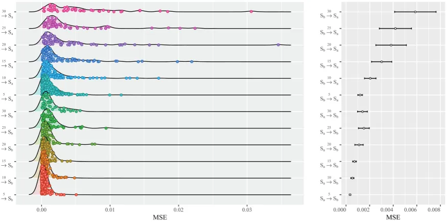
In Fig.5a, we show the distribution of the MSE obtained in the prediction simulations of SVR in the different prediction periods and time seriesSa andSb, which will allow us to evaluate the capabilities of prediction statistically. In addition, the confidence intervals are shown in Fig.5b, with a 5% significance for the mean estimation of the MSE of the sample obtained from the simulation. That is, intervals built at 95% confidence.

Jan Mar May Jul Sep Nov _Jan 2017 0.7 Price 0.6 0.5 0.4

Figure 4.Example of a five-day prediction in 2017. The solid line is the original series. The dotted line is the prediction.

● ● ● ● ● ●●●●● ●●●● ●●●●● ● ● ●● ● ● ● ● ● ● ● ●● ● ● ● ● ● ●● ● ● ●● ● ● ● ● ● _● ● ● ● ● ● ● ● ● ● ● ● ● ● ● _● ● ● ● ● ● ● ● ●● ● ● ●_● ●● ● ● ● ● ● ● ● ● ● ● ● ●● ● ● ● ● ● ● ● ● ● ● ● ● ● ● ● ● ● ● ● ● ● ● ● ● ● ● ● ● _● ● ● ● ● _● ●● ● _● ● _● ●● ●● ● ● ● ● ● ● ● ● ●● ● ● ● ● ● ● ● ● ● ● ● ● ● ● ● ● ● ● ● ● ● ● ● ● ●●● ● ● ● ● ● ● ● ● ● ● ● ● ● _● ● ● ● ● ● ● ● ● ● ●● ● ● ● ● ●● ● ● ● ●● ● ● ● ● ● ● ● ● ● ● ● ● ● ● ● ●● ● ● ● ● ● ● ● ● ● ● ● ● ● ● ● ● ●● ● ● ● ● ● ● ● ● ● ● ● ● ● ● ● ● ●●●●●● ● ● ● ● ● ● ● ● ● ● ● ●● ●_●● ● ● ● ● ● ● ● ● ● ● ● ● ● ● ● ● ● ● ● _● ● ● ● ● ● ● ● ● ● ● ● ● ● ● ● ● ●● ● ● ● ● ● ● ● ● ● ● ●● ● ● ●●● ● ● ● ● ● ● ● ● ● ● ● ● ● ●● ● ● ● ● ● ● ● ● ●●● ● ● ● ● ● ● ● ● ● ● ●●●●● ● ● ● ● ● ●● _● ● ● ● ●● ● ● ● ● ● ● ● ● ● ● ● ● ● ● ● ● ● ●●● ● ●●● ● ● ● ● ● ●●●● ● ● ● ● ● ● ● ● ● ●●● ● ●●●●●●●●●●●●●●●●●●●●●● ● ● ● ●●●●● ●●●●●●●● ●●●●●●●●● ● ●●●●●●●●●● ● ●●●●●●●●●●●●●●●●●●●● ● ●●●● ● ● ● ●●● ●●●●●●●●●●●●●●●●●●●●●●●●●●●●●●●●●● ● ● ● ● ● ● ● ● ● ● ● ● ● ● ● ● ●● ● ● ● ● ● ● ● ● ● ● ● ● ● ● ● ● ● ● ●● ● ● ● ● ● ● ● ● ● ● ● ● ● ● ● ● ● ● ● ●● ● ● ● ● ● ● ● ●● ●● ● ● ● ● ● ● ● ● ● ● ●● ● ● ● ● ● ● ● ● ● ● ● ● ●● ● ● ● ● ● ● ● ●● ● ● ● ● ● ● ● ● ● ● ● ● ● ● ● ● ● ● ● ● ● ● ● ● ●● ● ● ● ● ● ●●● ● ● ● ● ● ● ●● ● ● ● ● ● ● ● ● ● ● ● ● ●● ● ● ● ● ● ● ●●● ● ● _● ● ● ● ● ● ● ● ● ● ● ● ● ● ● ●● ● ● ● ● ● ● ● ● ● ● ● ● ● ●● ● ● ● ● ● ● ● ● ● ● ● ● ● ● ● ● ● ● ● ● ● ● ● ●● ● ● ● ● ● ●● ● ● ● ● ● ● ● ● ● ● ● ● ● ● ● ● ● ● ● ●●●●●●●●●●●●●●●●●●●●●●●●●●●●●●●●●●●●●●●●●●●●●●●●●●●●●●●●●●●●●●●●●●●●●●●●●●●●●_●●●●●●●●●●●●●●●●●●●●●● ● ● ● ● ● ●●●●●●●●●● ● ●●●●●●●●●●●●●●●●●●●●●●●●●●●●●●●●●●●●●●●●●●●●●●●●●●●●●●●●●●●●●●●●●●●●●●●●●●●●●●●●●●●●●●●●●●●●●●●●●●●●●●●●●●●●●●●●●●●●●●●●●●●●●_{● ●●●●●●●●●●●●●●●●●●}●●●●●●●●●●●●●●●●●●●●●●●●●●●●●●●●●●●●●●●●●●●●●●●●●●●●●●●●●●●●●●●●●●●●●●●●●●●●●●●●●●●●●●●●●●●●●●●●●●●●●●●●●●●●●●●●●●●●●●●●●●●●●●●●●●●●●●●●●●●●●●●●●●●●●●●●●●●●●●●●●●●●●●●●●●●●●●●●●●●●●●●●●●●●●●●●●●●●●●●●●●●●●●●●●●●●●●●●●●●●●●●●●●●●●●●●●●●●●●●●●●●●●●●●●●●●●●●●●●●●●●●●●●●●●●●●●●●●●●●●●●●●●●●●●●●●●●●●●●●●●●●●●●●●●●●●●●●●●● ● ● ● ● ● ● ● ● ● ●● ● ● ● ● ● ● ● ● ● ● ● ● ● ● ● ● ●● ●● ● ● ● ● ●● ● ● ● ● ● ● ● ● ● ● ● ●●● ● ●● ● ● ●_{● ●} ● ●● ● ● ● ● ● ● ● ● ● ● ● ● ● ● ●● ● ● ● ● ● ● ● ● ● ● ● ● ● ● ● ● ● ● ● ● ● ● ● ● ● ● ● ● ● ● ● ● ● ● ● ● ● ● ● ● ● ● ● ● ●●● ●●●●_●●● ● ● ●●● ●●●●●●●●●●●●●●_{●●●●●●●●}●●●●●●●●_{●●●●●}● ● ● ● ●●●●●● ●●● ● ● ●●● ● ●● ● ●●● ●●●●●●● ● ●●●●● ● ●●●●●●●● ● ● ● ● ●●●●●●● ● ●●●●●●● ● ●●●● ●●●●●●●●●●● ●● ●●●● ●● ● ● ● ●● ● ● ● ● ● ● ●● ● ● ● ● ● ● ● ● ● ● ● ● ● ● ● ● ● ● ● ● ● ● ● ● ● ● ● ● ● ● ● ● ● ● ● ● ● ● ● ● ●● ● ● ● ● ● ●●_● ● ● ● ● ● ●● ● _● ● ● ●● ● ● ● ●● ● ● ● ● ● ● ● ● ● ● ● ● ● ● ● ● ● ● ● ● ● ● ● ● ● ● ● ● ●● ● ● ● ● ● ● ● ●●●●●●●●●●● ● ● ● ● ●●●●●●●●●●●●● ● ● ● ●●● ● ●● ● ● ● ● ● ●●●●●● ● ● ● ● ● ● ● ● ● ● ●●● ● ● ● ● ● ● ● ● ● ● ● ● ● ● ● ● ● ● ● ● ● ● ●●●● ● ● ● ● ● ● ● ● ● ●●●●●●●●●●●●●●● ● ● ● ● ●●●●●●●●●●●●● ●●●●●● ● ●●●●●●●●●_●●●●●●●_●●● ● ●●●●●●●●●●●●●●●●●●●●●●●●●● ● ● ● ● ● ● ● ● ● ● ● ● ●●●●● ● ● ●●● ● ●● ● ● ● ● ● ● ●●●●●●●●●● ● ●●●●●● ● ● ● ● ● ● ● ●●●● ● ●●●● ● ●●_{●●●●●●●●●}●●●●●●●●●●●●●●●●●●●●●●●●●●●●●●●●●●●●●●●●●●●●●●●●●●●_●● ● ● ● ● ● ●●●●●●●●● ●●● ● ●● ●● ● ●●● ● ● ● ●● ● ● ● ● ● ● ● ● ● ● ● ● ● ● ● ● ● ● ● ● ● ● ● ● ● ● ● ● ● ● ●●● ● ● ● ● ● ● ● ● ● ● ● ● ● ● ● ● ● ● ● ● ● ● ● ● ● ● ● ● ● ● ●● ● ● ● ● ● ● ● ● ● ● ● ● ● ● ● ● ● ● ● ● ● ●● ● ● ● ● ● ● ● ● ● ● ● ● ● ● ● ● ● ● ● ● ●● ●●●●●●●●●●●● ● ● ● ● ● ● ● ● ● ● ● ● ● ● ● ● ● ● ● ● ● ● ● ● ● ● ● ● ●●●●● ● ● ● ● ●●●●●●●●●●●●●●●●●●●●●●● ● ●● ●●●●●●●●●●●●●●●●●●●●●●●●●●●●● ● ● ● ●●●●●●●●●●● ● ●●● ●●●●●●●●●●●●●●●●●●●● ● ●●●●●●●●●●●●●●●●●●●●●●●●●●●●●●●●●●●●●●●●●●●●●●●●●●●●●●●●●●●●●●●●●●●●●●●●●●●●●●●●●●●●●●●●●●●●●●●●●●●●●●●●●●●●●●●●●●●●●_●●●●●●●●●●●●●●●●●● ● ●●●●●●●●●●●●●●● ● ● ● ●●●●●● ● ●● ● ●●●●●●●●●●●●●●●● ● ● ● ● ● ● ●●●●●●●●●●●●●●●●●●●●●●●●●●●●●●●●●●●●●●●●●●●●●●●●●●●●●●●●●●●●●●●●●●●●●●●●●●●●●●●●●●●●●●●●●●●●●●●●●●●●●●●●●●●●●●●●●●●●●●●●●●●●●●●●●●●●●●●●●●●●●●●●●●●●●●●●●●●●●●●●●●●●●●●●●●●●●●●●●●●●●●●●●●●●●●●●●●●●●●●●●●●●●●●●●●●●●●●●●●●●●●●●●●●●●●●● ● ●●●●●●●●●●●●●●●●●●●●●●●●● ● ● ● ● ● ● ●●●●●●_{●●●●●●●●●●●●●●●●●●●●●●●●●●●●●}●●●●●●●●●●●●●●●●●●●●●●●●●●●●●●●●●●●●●●● ● ● ● ● ● ● ● ● ● ● ● ● ● ● ● ● ● ● ● ● ● ● ● ● ● ● ● ● ● ●●●●●●●●●●●●●●●●●●●●●●●●●●●●●●●●●●●●●●●●●●●●●●●●●●●●●●●●●●●●●●●●●●●●●●●●●●●●●●●●●●●●●●● ● ● ● ● ● ● ● ● ● ● ● ● ● ● ●●●●●●●●●●●●●●●●●●●●● ● ● ● ● ● ● ● ●●●●●●●●●●●●●●●●●●●●●●●●●●●●●●●●● ●●●●●●●●●●●●●●●●●●●_{●●●●●●●●●●●●●●●●●}●●●●●●●●●●●●●●●●●●●●●●●●●●●●●●●●●●●●●●●●●●●●●●●●●●●●●●●●●●●●●●●●●●●●●●●●●●●●●●●●●●●●●●●●●●●●●●●●●●●●●●●●_● ● ● ● ● ● ● ● ● ● ● ● ● ● ● ● ● ● ● ●●_●●●●● ● ● ● ● ● ● ●●●●●●●●●●●●●●●●●● ● ● ● ● ● ● ●●●●●●●●● ● ●●● ● ● ●●●●●●● ● ● ● ● ● ● ● ● ● ● ● ● ● ●● ● ● ● ● ● ● ● ● ● ● ● ● ● ● ● ● ● ● ● ●● ● ● ● ● ● ● ● ● ● ● ● ● ● ● ● ● ● ●● ● ● ● ● ● ● ● ● ●● ●●● ● ● ● ● ● ● ● ● ● ● ● ● ● ● ● ● ● ● ●●● ● ● ● ● ● ● ● ● ● ● ● ● ● ● ● ● ● ● ● ● ● ● ● ●● ● ● ● ● ● ● ● ● ● ● ● ● ● ●● ● ● ● ● ● ● ●_● ●●●● ● ● ● ● ● ● ● ● ● ●●●●● ● ●●●●● ● ● ● ● ● ● ● ● ● ● ● ● ● ● ● ● ● ● ● ● ● ● ● ● ● ●●●●●●● ● ● ● ● ● ● ● ● ●●●●● ● ●● ● ● ● ●●● ● ● ● ● ● ● ● ● ● ● ● ● ● ● ● ● ● ● ● ● ● ● ● ● ● ● ● ● ● ● ● ● ● ● ● ● ● ● ● ● ● ● ● ● ● ● ● ● ● ● ● ● ● ● ● ● ● ● ● ● ● ● ● ● ● ● ● ● ●●●●●●●●●●●●●●●● ● ● ● ● ● ● ● ● ● ● ● ● ● ● ● ● ● ● ● ● ● ● ● ● ● ● ● ● ● ● ● ● ● ● ● ● ● ● ● ● ●●●●●●_●●●●●●●●●●●●●●●●●●●●●● ● ● ● ● ● ● ● ● ● ● ● ● ● ● ● ● ● ● ● ● ● ● ● ● ● ● ●●●●●●●●●●●●●●●●● ● ● ● ● ● ● ● ● ● ● ● ● ● ● ●●● ● ●●●● ● ● ● ● ● ● ●●●●●●●●●●●●●●●●●●●●●●●●●●●●●●●●●●●● ●●●●●●●●●●●●●●● ● ● ●●●●●●●●●●●●●●●●●●●●●●●●●● ● ● ● ● ● ● ● ● ● ● ● ● ● ● ●●●●●●●●●●●●●●●●●●●●●●●●●●●●●●●● ● ● ● ● ● ● ● ● ● ● ● ● ●●●●●●●●●●●●● ● ● ● ● ●●●●●●●●●●●●●●●●●●●●● ● ● ● ● ● ● ●●●●● ● ●●_{●●●●●●●●●●●}● ● ● ● ● ● ● ●●●●●●●●●●●●●●●●●●●●●●●●●●●●●●●●●●●●●●●●●●●●●●●●●●●●●●●●●●●●●●●●●●●●●●●●●●●●●●●●●●●●●●●●●●●●●●●●●●●●●●●●●●●●●●●● ● ●●●●● ● ● ● ● ●●● ● ● ●● ● ● ● ● ● ● ● ● ● ● ● ● ● ● ● ● ● ● ● ● ● ● ● ● ● ● ● ● ● ● ●●●●●●●●●●●●●●●●●●●●●●●●●●●●●●●●●●●●●●●●●●●●●●●●●●●●●●●●●●●●●●●●●●●●●●●●●●●●●●●●●●●●●●●●●●●●●●●●●●●●●●●●●●●●●●●●●●●●●●●●●●●●●●●●●●●●●●●●●●●●●●●●● ● ● ● ● ● ● ● ● ● ● ● ● ● ● ● ● ● ● ● ● ● ● ● ● ● ● ● ● ● ●●●●●●●●●●●●●●●●●●●●●●●●●●●●●●●●●●●●● ● ● ● ● ● ● ● ● ● ● ● ● ● ●●●●●●●●●●●●●●●●●●●●●●●●●●●●●●● ● ● ● ●●●●●●●●●●●● ● ● ● ● ● ● ●●●●●● ● ●● ● ● ● ● ● ● ● ● ● ● ● ● ● ● ● ● ● ● ● ●●●●●●●●● ● ● ● ● ● ● ● ● ● ● ● ● ● ● ● ● ● ● ● ● ● ● ● ● ● ● ● ● ● ● ● ● ● ● ● ● ● ● ● ● ● ● ● ● ● ● ● ● ● ● ● ● ● ● ● ● ● ● ● ● ● ● ● ● ● ● ● ● ● ● ● ● ● ● ● ● ● ● ● ● ● ● ● ● ● ● ● ● ● ● ● ● ● ● ● ● ● ● ● ● ● ● ● ● ● ● ● ● ● ● ● ● ● ● ● ● ● ● ● ● ● ● ● ● ● ● ● ● ● ● ● ● ● ● ● ● ● ● ● ● ● ● ● ● ● ● ● ● ● ● ● ● ● ● ● ● ● ● ● ● ● ● ● ● ● ● ● ● ● ● ● ● ● ● ● ● ● ● ● ● ● ● ● ● ● ● ● ● ● ● ● ● ● ● ● ● ● ● ● ● ● ● ● ● ● ● ● ● ● ● ● ● ● ● ● ● ● ● ● ● ● ● ● ● ● ● ● ● ● ● ● ● ● ● ● ● ● ● ● ● ● ● ● ● ● ● ● ● ● ● ● ● ● ● ● ● ● ● ● ● ● ● ● ● ● ● ● ● ● ● ● ● ● ● ● ● ● ● ● ● ● ● ● ● ● ● ● ● ● ● ● ● ● ● ● ● ● ● ● ● ● ● ● ● ● ● ● ● ● ● ● ● ● ● ● ● ● ● ● ● ● ● ● ● ● ● ● ● ● ● ● ● ● ● ● ● ● ● ● ● ● ● ● ● ● ● ● ● ● ● ● ● ● ● ● ● ● ● ● ● ● ● ● ● ● ● ● ● ● ● ● ● ● ● ● ● ● ● ● ● ● ● ● ● ● ● ● ● ● ● ● ● ● ● ● ● ● ● ● ● ● ● ● ● ● ● ● ● ● ● ● ● ● ● ● ● ● ● ● ● ● ● ● ● ● ● ● ● ● ● ● ● ● ● ● ● ● ● ● ● ● ● ● ● ● ● ● ● ● ● ● ● ● ● ● ● ● ● ● ● ● ● ● ● ● ● ● ● ● ● ● ● ● ● ● ● ● ● ● ● ● ● ● ● ● ● ● ● ● ● ● ● ● ● ● ● ● ● ● ● ● ● ● ● ● ● ● ● ● ● ● ● ● ● ● ● ● ● ● ● ● ● ● ● ● ● ● ● ● ● ● ● ● ● ● ● ● ● ● ● ● ● ● ● ● ● ● ● ● ● ● ● ● ● ● ● ● ● ● ● ● ● ● ● ● ● ● ● ● ● ● ● ● ● ● ● ● ● ● ● ● ● ● ● ● ● ● ● ● ● ● ● ● ● ● ● ● ● ● ● ● ● ● ● ● ● ● ● ● ● ● ● ● ● ● ● ● ● ● ● ● ● ● ● ● ● ● ● ● ● ● ● ● ● ● ● ● ● ● ● ● ● ● ● ● ● ● ● ● ● ● ● ● ● ● ● ● ● ● ● ● ● ● ● ● ● ● ● ● ● ● ● ● ● ● ● ● ● ● ● ● ● ● ● ● ● ● ● ● ● ● ● ● ● ● ● ● ● ● ● ● ● ● ● ● ● ● ● ● ● ● ● ● ● ● ● ● ● ● ● ● ● ● ● ● ● ● ● ● ● ● ● ● ● ● ● ● ● ● ● ● ● ● ● ● ● ● ● ● ● ● ● ● ● ● ● ● ● ● ● ● ● ● ● ● ● ● ● ● ● ● ● ● ● ● ● ● ● ● ● ● ● ● ● ● ● ● ● ● ● ● ● ● ● ● ● ● ● ● ● ● ● ● ● ● ● ● ● ● ● ● ● ● ● ● ● ●●●●●●●● ● ● ● ● ● ● ●●●●●●●●● ● ●●● ● ● ● ● ● ● ● ● ● ● ● ● ● ●●● ● ● ● ● ● ● ● ● ● ● ● ● ● ● ● ● ●●●●● ● ●●●●●●●●●●●●●●●●●●●● ● ●●●●●●●●●●●●●●●●● ● ●●●●●●●●●●●●●●●●●●●●●●●●●●●●● ● ● ● ● ● ● ● ● ● ● ● ● ● ●●●●●●●●●●● ● ● ● ● ● ● ●●●● ● ● ● ● ● ●●●●●●●●●●●●●●●●●●●●● ● ●●●●●●●● ● ●●●●●●● ● ●●●●● ● ● ● ● ● ● ● ● ● ● ● ● ● ● ● ● ● ● ● ● ● ● ● ● ● ●●●●●●_● ● ●●●●● ● ● ● ●●●●●●●●●●●●●●●●●●●●●●●●●●●●●●●●●●●●●●●●●●●●●●●●●●●●●●●●●●●●●●●●●●●●●●●●●●●●●●●●●●●●●●●●●●●●●●●●●●●●●●●●●●●●●●●●●●●●●●●●●●●●●●●●●●●●●●●●●●●●●●●●●●●●●●●●●●●●●●●●●●●●●●●●●●●●●●●●●●●●●●●●●●●●●●●●●●●●●●●●●●●●●●●●●●●●●●●●●●●●●●●●●●●●●●●●●●●●●●●●●●●●●●●●●●●●●●●●●●●●●●●●●●●●●●●●●●●●●●●●●●●●● ● ● ● ● ● ● ● ● ● ● ● ● ● ● ● ● ● ● ●●●●●●●●●●● ● ● ●●● ● ● ● ● ● ● ●●●●●●●●●●●●●●● ● ● ● ●●●●●●●●●●●●●●●●● ● ● ● ●●●●●●●●●●●●●●●●●●●●●●●●●●●●●●●●●●●●●●●●●●●●●●●●●●●●●●●●●●●●●●●●●●●●●●●●●●●●●●●●●●●●●●●● ● ● ● ● ● ● ● ● ● ● ● ● ● ● ●●●●●●●●●●●●●●●●●●●●●●●●●●●●●●●●●●● ●●●●●●●●●●●●●●● ● ● ●●●●●●●●●●●●●●●●●●●●●●●●●●●●●●●●●●●●●●●● ●●● ● ● ● ● ● ● ● ● ● ● ● ● ● ● ●●●●●●●● ● ● ● ●●●●●●●●●●●●●●●●●●●●●●●●●●●●●●●●●●●●●●●●●●●●●●●●●●●●●●●●●● ● ● ● ● ● ● ● ● ● ● ● ● ● ●●●●●●●●●●●●●●●●●●●●●●●●●●●●●●●●●●●●●●●●●●●●●●●●●●●●●●●●●●●●●●●●●● ● ● ● ●●●●●●●●●●●●●●●●●●●●●●●●●●●●●●●●●●●●●●●●●●●●●●●_{●●●●●●●●●●●●●●●●●●●●●●●●●●●●●}●●●●●●●●●●●●●●●●●●●●●●●●●●●●●●●●●●●●●●●●●●●●●●●●●●●●●●●●●●●●●●●●●●●●●●●●●●●●●●●●●●●●●●●●●●●●●●●●●●●●●●●●●●●●●●●●●●●●●●●●●●●●●●●●●●●●●●●●●●●●●●●●●●●●●●●●●●●●●●●●●●●●●●●●●●●●●●●●●●●●●●●●●●●●●●●●●●●●●●●●●●●●●●●●●●●●●●●●●●●●●●●●●●●●●●●●●●●●●●●●●●●●●●●●●●●●●●●●●●●●●●●●●●●●●●●●●●●●●●●●●●●●●●●●●●●●●●●●●●●●●●●●●●●●●●●●●●●●●●●●●●●●●●●●●●●●●●●●●●●●●●●●●●●●●●●●●●●●●●●●●●●●●●●●●●●●●●●●●●●●●●●●●●●●●●●●●●●●●●●●●●●●●●●●●●●●●●●●●●●●●●●●●●●●●●●●●●●●●●●●●●●●●●●●●●●●●●●●●●●●●●●●●●●●●●●●●●●●●●●●●●●●●●● ● ● ●●●●●●●●●●●●●●●●●●●●●●●●●●●●●●●●●●●●●●●●●●●●●●●●●●●●●●●●●●●●●●●●●●●●●●●●●●●●●●●●●●●●●●●●●●●●●●●●●●●●●●●●●●●●●●●●●●●●●●●●●●●● ● ● ● ● ● ● ● ●●●●●●●● ● ● ● ● ● ● ● ●●●●●●●●● ● ● ● ● ● ● ● ● ● ● ● ● ● ● ● ● ● ● ● ●●●●●●●●●●●●●●●●●●●●●●●●●●●●● ● ● ● ● ● ● ● ● ● ● ● ● ● ● ●●●●●●●●●●●●●●●●●●● ● ● ● ● ● ● ● ● ● ● ● ● ● ●●●●●●●●●●●●●●●●●●● ● ● ● ● ● ● ●●●●●●●●●●●●●●●●●●●●●●●●●●●●●●●●●●●●●●●● ● ● ● ● ● ● ● ● ● ● ● ● ● ● ● ● ● ● ● ● ● ● ● ● ● ● ● ● ● ● ● ● ● ● ● ● ● ● ● ● ● ● ● ● ● ● ● ● ● ● ● ● ● ● ● ● ● ● ● ● ● ● ● ● ● ● ● ● ● ● ● ● ● ● ● ● ● ● ● ● ● ● ● ● ● ● ● ● ● ● ● ● ● ● ● ● ● ● ● ● ● ● ● ● ● ● ● ● ● ● ● ● ● ● ● ● ● ●●●●●●●●●●●●●●●●●●●●●●●●●●●●●●●●●●●●●●●●●●●●●●●●●●●●●●●●●●●●●●●●●●●●●●●●●●●●●●●●●●●●●●●●●●●●●●●●●●●●●●●●●●●●●●●●●●●●●●● ● ● ● ● ● ● ●●●●●●●●●●●●●● ● ● ● ●●●●● ●●●●●●●●●●●●●●●●●●●●● ● ● ● ● ● ● ● ● ● ● ● ● ● ● ● ● ● ● ● ● ● ● ● ● ● ● ● ●● ● ● ● ● ● ●● ●● ● ● ● ● ● ● ● ●●● ● ● ● ● ● ● ●●_● ● ● ● ● ● ● ● ● ● ● ● ● ● ● ● ● ● ●● ●● ● ● ● ● ● ● ●● ● ● ● ● ● ● ● ● ● ● ● ● ● ● ● ● ●● ● ● ● ● ● ● ● ● ● ● ● ● ● ● ● ● ● ● ● ● ● ● ● ●● ● ● ● ● ● ● ● ● ● ● ● ● ● ● ● ● ● ● ● ● ● ●● ● ● ● ● ● ●● ● ● ● ● ● ● ● ● ●● ●● ● ● ● ● ● ● ● ● ● ● ● ● ● ● ● ●● ● ● ● ● ● ● ● ● ●● ● ● ● ● ● ● ● ● ● ● ● ● ● ● ● ● ● ● ● ● ● ● ●● ●● ● ● ● ● ● ● ● ● ● ● ● ●● ● ● ● ● ● ● ● ● ● ●● ● ● ● 6D→6E

6D→6E

6D→6E

6D→6E

6D→6E

6D→6E

6E→6D

6E→6D

6E→6D

6E→6D

6E→6D

6E→6D

06(

(a)Distribution MSE for type and interval.

● ● ● ● ● ● ● ● ● ● ● ● ● ● ● ● ● ● ● ● ● ● ● ● 5

Sa→ Sb 1 0

Sa→ Sb 1 5

Sa→ Sb 2 0

Sa→ Sb 2 5

Sa→ Sb 3 0

Sa→ Sb 5

Sb→ Sa 1 0

Sb→ Sa 1 5

Sb→ Sa 2 0

Sb→ Sa 2 5

Sb→ Sa 3 0

Sb→ Sa

0. 0 0 0 0. 0 0 2 0. 0 0 4 0. 0 0 6 0. 0 0 8

M S E

(b) 95% Family-wise confidence level.

Figure 5.MSE.

Table 3. p-value; ., *, **, *** indicate statistical significance at the 90%, 95%, 99% and 99.9% levels respectively.

Sa→5 Sb Sa→10Sb Sa→15Sb Sa→20Sb Sa→25Sb Sa→30Sb Sb→5 Sa Sb→10Sa Sb→15Sa Sb→20Sa Sb→25Sa Sb→30Sa

Sa→5 Sb . * *** *** *** *** ***

Sa→10Sb 0.999905 *** *** *** *** ***

Sa→15Sb 0.989177 0.999996 ** *** *** *** ***

Sa→20Sb 0.558148 0.943909 0.998648 *** *** *** ***

Sa→25Sb 0.085021 0.412852 0.800756 0.999168 * *** *** ***

Sa→30Sb 0.301065 0.723441 0.950625 0.999984 0.999999 * *** *** ***

Sb→5 Sa 0.014257 0.430887 0.936813 0.999999 0.999582 0.999998 . *** *** *** ***

Sb→10Sa 8.12e-08 0.000129 0.008314 0.345577 0.977224 0.939273 0.098575 *** *** ***

Sb→15Sa 4.53e-13 2.13e-10 1.62e-07 0.000211 0.029091 0.023743 1.06e-06 0.213923 ***

Sb→20Sa 4.37e-13 4.34e-13 6.78e-12 4.79e-08 4.55e-05 4.85e-05 1.70e-11 0.000316 0.744952 **

Sb→25Sa 4.37e-13 4.21e-13 9.94e-13 3.43e-09 3.69e-06 4.16e-06 2.25e-12 2.34e-05 0.271314 0.999789 .

7. Discussion

The MSE presented in Table2corresponds to the total error of the prediction in comparison with the real data. The dispersion of the error is obtained from the forecast in each one of these intervals. It is made eachpjof days. This situation is presented in Fig.5a.

Another characteristic important to mention with respect to the errors is, when trained with the oldest series of time, the dispersion of the errors is less compared to the training based with the most recent part of the series. Table2shows that the RMSE error for the 30-day prediction is 3.30% when training with theSaseries.

Our results show that the presented model is able to predict copper price volatilities near reality. Similar results are obtained in other works, such as the work presented in [31]. In this work, a bat algorithm was used[32] to determine the coefficients of time series functions to predict the behaviour of the same time series of this work, but exclusively during the year 2016. To do this, training with data from 2009 until 2015 was performed. Under those conditions, the prediction error isRMSE=1.36%. With the method proposed in this paper, an error ofRMSE=1.42% is achieved.

Finally, we can observe in Fig.5athat there are significant differences of the MSE at 95% confidence, betweenSa → Sb andSb → Sa in each of the prediction intervals 5, 10, 15, 20, 25 and 30 days. In contrast, for the prediction Sa → Sb there are no significant differences in the MSE between the prediction intervals 5, 10, 15, 20, 25 and 30 days. This allows us to show the robustness of the prediction in the short and medium-term since the prediction at the 5-day interval has not lost performance over the 30-day prediction interval considering it in this case as a medium-term. This is useful for the decision-making process for mining companies and traders. On the other hand, to affect the decision-making process for investors and the government, it is necessary to have reliable long-term forecasts.

8. Conclusions

In this work, the construction of a model was presented based on SVR that allows making a prediction of the closing value of copper in the Metal London Stock Exchange, being the RMSE equal or less than the 2.2% for prediction periods of 5 and 10 days. The method consists of finding the best model through a search in a grid, wherein each model is trained and tested through use of the balancing methods in cross-validation. For the training process, only the data of closing price of the series is used. The results indicate that the model of the SVR regardless of the number of days of the prediction, and this can be done having three actual values. Additionally, we observed that more current data negatively impact on the MSE. This phenomenon must be studied in the future, but there is a signal that this can be explained through the level of noise and the amount of data of the training time series.

The importance of price prediction will depend on the interest of the agents and their objectives, in short, medium and long-term prediction periods. Our work aims for short-term predictions of 5 days, 10, . . . , up to 30 days. These predictions will interest brokers and investors who seek to take advantage of the periodic variations with active portfolio management. For medium-term predictions, such as monthly and annual, governments may be more interested in their national budget, as is the case in Chile, which is an economy whose income and tax revenues come from copper mining. In the long-term, more than one year. Investors and mining companies will be more interested in their long-term investment plans, such as, the process of improvement, expansion, a search of new deposits that give value to their investments, or institutional or private investors, with long-term investment horizons withbuy and holdinvestment strategies.

Author Contributions: Conceptualization, Gabriel Astudillo, Raúl Carrasco and Máx Chacón; Formal analysis, Gabriel Astudillo; Funding acquisition, Máx Chacón; Investigation, Gabriel Astudillo and Raúl Carrasco; Methodology, Gabriel Astudillo, Raúl Carrasco, Christian Fernández-Campusano and Máx Chacón; Project administration, Máx Chacón; Software, Gabriel Astudillo and Raúl Carrasco; Supervision, Máx Chacón; Validation, Christian Fernández-Campusano; Visualization, Gabriel Astudillo and Raúl Carrasco; Writing – original draft, Gabriel Astudillo and Raúl Carrasco; Writing – review & editing, Christian Fernández-Campusano.

Acknowledgments:We are grateful to the Universidad de Santiago de Chile (USACH) and to Parcialy founded

for Fondecyt project #1181659. Furthermore, the authors thank Paul Soper for the style correction of the language.

Conflicts of Interest:The authors declare that there is no conflict of interest in the publication of this paper.

References

1. Oglend, A.; Asche, F. Cyclical non-stationarity in commodity prices. Empirical Economics 2016,

51, 1465–1479. doi:10.1007/s00181-015-1060-6.

2. Lasheras, F.S.; de Cos Juez, F.J.; Sánchez, A.S.; Krzemie ´n, A.; Fernández, P.R. Forecasting the COMEX copper spot price by means of neural networks and ARIMA models. Resources Policy2015,45, 37–43. 3. Ebert, L.; Menza, T.L. Chile, copper and resource revenue: A holistic approach to assessing commodity

dependence. Resources Policy2015,43, 101 – 111.

4. Spilimbergo, A. Copper and the Chilean Economy, 1960-98. Policy Reform 2002, 5, 115–126.

doi:10.1080/13841280290015646.

5. Kriechbaumer, T.; Angus, A.; Parsons, D.; Rivas Casado, M. An improved wavelet-ARIMA approach for forecasting metal prices. Resources Policy2014,39, 32–41. doi:10.1016/j.resourpol.2013.10.005.

6. Seguel, F.; Carrasco, R.; Adasme, P.; Alfaro, M.; Soto, I. A Meta-heuristic Approach for Copper Price Forecasting. InInformation and Knowledge Management in Complex Systems; Liu, K.; Nakata, K.; Li, W.; Galarreta, D., Eds.; Springer International Publishing: Toulouse, France, 2015; Vol. 449,IFIP Advances in Information and Communication Technology, pp. 156–165. doi:10.1007/978-3-319-16274-4\_16.

7. Carrasco, R.; Vargas, M.; Alfaro, M.; Soto, I.; Fuertes, G. Copper Metal Price Using Chaotic Time Series Forecating. IEEE Latin America Transactions2015,13, 1961–1965. doi:10.1109/TLA.2015.7164223.

8. Carrasco, R.; Vargas, M.; Soto, I.; Fuentealba, D.; Banguera, L.; Fuertes, G. Chaotic time series for copper’s price forecast: neural networks and the discovery of knowledge for big data. InDigitalisation, Innovation, and Transformation; Liu, K.; Nakata, K.; Li, W.; Baranauskas, C., Eds.; Springer, Cham: London, UK, 2018; Vol. 527, pp. 278–288. doi:10.1007/978-3-319-94541-5\_28.

9. Khalifa, A.; Miao, H.; Ramchander, S. Return distributions and volatility forecasting in metal futures markets: Evidence from gold, silver, and copper. Journal of Futures Markets2011, 31, 55–80. doi:10.1002/fut.20459.

10. Cortazar, G.; Eterovic, F. Can oil prices help estimate commodity futures prices? The cases of copper and silver. Resources Policy2010,35, 283–291. doi:10.1016/j.resourpol.2010.07.004.

11. Cortazar, G.; Kovacevic, I.; Schwartz, E.S. Commodity and asset pricing models: An integration. Technical report, National Bureau of Economic Research, 2013.

12. Fernandez-Perez, A.; Fuertes, A.M.; Miffre, J. Harvesting Commodity Styles: An Integrated Framework.

INFINITI conference on International Finance2017.

13. Jaramillo, J.A.; Velásquez, J.D.; Franco, C.J. Research in Financial Time Series Forecasting

with SVM: Contributions from Literature. IEEE Latin America Transactions 2017, 15, 145–153. doi:10.1109/TLA.2017.7827918.

14. Vapnik, V. The Nature of Statistical Learning Theory; Springer, New York, NY, 1995; p. 188.

doi:10.1007/978-1-4757-2440-0.

15. Drucker, H.; Burges, C.J.; Kaufman, L.; Smola, A.; Vapnik, V. Support vector regression machines. Advances in neural information processing systems1997,9, 155–161. doi:10.1.1.10.4845.

16. Vapnik, V.; Golowich, S.E.; Smola, A.J. Support Vector Method for Function Approximation, Regression Estimation and Signal Processing. InAdvances in Neural Information Processing Systems 9; Mozer, M.C.; Jordan, M.I.; Petsche, T., Eds.; MIT Press, 1997; pp. 281–287.

18. Kao, L.J.; Chiu, C.C.; Lu, C.J.; Chang, C.H. A hybrid approach by integrating wavelet-based feature extraction with MARS and SVR for stock index forecasting. Decision Support Systems2013,54, 1228–1244,

[arXiv:1011.1669v3]. doi:10.1016/j.dss.2012.11.012.

19. Kazem, A.; Sharifi, E.; Hussain, F.K.; Saberi, M.; Hussain, O.K. Support vector regression with chaos-based firefly algorithm for stock market price forecasting. Applied Soft Computing Journal2013,13, 947–958. doi:10.1016/j.asoc.2012.09.024.

20. Patel, J.; Shah, S.; Thakkar, P.; Kotecha, K. Predicting stock market index using fusion of machine learning techniques.Expert Systems with Applications2014,42, 2162–2172. doi:10.1016/j.eswa.2014.10.031. 21. Cristianini, N.; Shawe-Taylor, J.; others. An introduction to support vector machines and other kernel-based

learning methods; Cambridge university press, 2000.

22. Shokri, S.; Sadeghi, M.T.; Marvast, M.A.; Narasimhan, S. Improvement of the prediction performance of a soft sensor model based on support vector regression for production of ultra-low sulfur diesel.Petroleum Science2015,12, 177–188. doi:10.1007/s12182-014-0010-9.

23. Chun-Hsin Wu.; Jan-Ming Ho.; Lee, D.T. Travel-time prediction with support vector regression. IEEE Transactions on Intelligent Transportation Systems2004,5, 276–281.

24. Yeh, C.Y.; Huang, C.W.; Lee, S.J. A multiple-kernel support vector regression approach for stock market price forecasting.Expert Systems with Applications2011,38, 2177 – 2186. doi:10.1016/j.eswa.2010.08.004. 25. Vert, J.P.; Tsuda, K.; Schölkopf, B. A primer on kernel methods.Kernel methods in computational biology2004,

47, 35–70.

26. Watkins, C.; McAleer, M. Econometric modelling of non-ferrous metal prices. Journal of Economic Surveys 2004,18, 651–701. doi:10.1111/j.1467-6419.2004.00233.x.

27. Hsu, C.W.; Chang, C.C.; Lin, C.J. A Practical Guide to Support Vector Classification. Technical report, National Taiwan University, Taipei, Taiwan, 2003.

28. McCarthy, P.J. The Use of Balanced Half-Sample Replication in Cross-Validation Studies. Journal of the American Statistical Association1976,71, 596–604. doi:10.1080/01621459.1976.10481534.

29. Meyer, D.; Dimitriadou, E.; Hornik, K.; Weingessel, A.; Leisch, F. e1071: misc functions of the department of statistics, probability theory group (formerly: E1071), TU Wien. R package version 1.6-7, 2015. 30. Analytics, R.; Weston, S. doParallel: Foreach parallel adaptor for the parallel package. R package version

2014,1.

31. Dehghani, H.; Bogdanovic, D. Copper price estimation using bat algorithm. Resources Policy2018. doi:10.1016/j.resourpol.2017.10.015.

32. Yang, X.S. A new metaheuristic Bat-inspired Algorithm. Studies in Computational Intelligence, 2010. doi:10.1007/978-3-642-12538-6_6.

Sample Availability:Samples of the compounds ... are available from the authors.

c