Video Transcoder in DCT-Domain Spatial Resolution Reduction Using Low-Complexity Motion Vector Refinement Algorithm

(1)

Volume 2008, Article ID 467290,15pages doi:10.1155/2008/467290

Research Article

Video Transcoder in DCT-Domain Spatial Resolution Reduction

Using Low-Complexity Motion Vector Refinement Algorithm

Tsung-Han Tsai, Yu-Fun Lin, and Hsueh-Yi Lin

Department of Electrical Engineering, National Central University, Jhongli, Taoyuan County 32001, Taiwan

Correspondence should be addressed to Hsueh-Yi Lin,[email protected]

Received 26 February 2008; Revised 30 June 2008; Accepted 2 September 2008

Recommended by Moon Kang

We address the topic of spatial-downscaling video transcoder in DCT-domain. The proposed techniques include the hierarchical fast motion resampling (HFMR) with accuracy motion resampling, the fast refinement for nonintegral (FRNI) motion vector (MV), and the dynamic regulating search (DRS) with low-complexity motion vector refinement. Two kinds of motion vector refinement algorithms in DRS are designed for diﬀerent architectures and applications. Based on brute-force motion compensation in DCT-domain (MC-DCT), FRNI can provide better quality than nonrefine MV and reduce the complexity. DRS can utilize the filter for half-pixel MV in MC-DCT and it is an eﬃcient method for extracting MC-DCT block to improve the performance further. From the experiments, the proposed algorithms can improve the entire quality and also reduce the complexity for DCT-domain video transcoder.

Copyright © 2008 Tsung-Han Tsai et al. This is an open access article distributed under the Creative Commons Attribution License, which permits unrestricted use, distribution, and reproduction in any medium, provided the original work is properly cited.

1. INTRODUCTION

Recently, the masses have brought up all kinds of multimedia services to more and more demands on digital video, such as video on demand, distance learning, and video surveillance. In these applications, compressed digital video is a major component of the multimedia data. Video coding technology makes those applications feasible. In video coding, an analog video signal is digitized and then compressed to fit into desirable bandwidth.

In the context of coding and transmission, there is an increasing need to perform many types of conversions to accommodate terminal constraints, network limitations, or preferences of user. There exists a rich set of contents that are rapidly growing by the day. On the other hand, we have terminals with varying capabilities. Connection between the terminals requires conversions to adapt between heterogeneous network configurations and the diﬀerences between terminal constraints. Among existing techniques, video transcoding has allowed user to convert a previously compressed bit-stream into another format to meet various multimedia services. The relative work is a process of converting a previously compressed video bit-stream into

another bit-stream with a lower bitrate, a diﬀerent resolution (e.g., downscaling), a diﬀerent coding format (e.g., the conversion between MPEG-x and H.26x, or adding error resilience), and so forth.

H.264 and H.263 play diﬀerent roles in current industry. H.264 is computationally expensive in software. Hardware realization can enhance the computation speed to achieve real-time goal. However, the real-time requirement on software is hard to achieve in H.264. If simple methods are applied, resulting performance might not be satisfactory. When real-time software is desired without considering too much performance gain, H.263 becomes an alternative. Especially in the age with wider Internet capacity, occupying larger bandwidth might be acceptable. Nowadays, most of existing mobile phones are capable of watching movies from 3GPP or MV4 format. Video clips from the phone-embedded camera are stored in 3GPP format. According to the general description, 3GPP is version of H.263 for streaming and mobile applications. Since it is widely adopted in mobile devices, transcoding between mobile phone can be conducted by H.263 transcoding.

(2)

MEM MC + + + IDCT

IQ2

End decoder

MEM FM

Encoder

Q2 DCT +

+

−

+ ₊+ IDCT

IQ2 MEM

MC

Decoder

IQ1 IDCT +

+ + Transcoder

MEM FM

Q1 DCT +

+

−

+ +

+ IDCT

IQ1 CIF

Front encoder

Figure1: A straightforward realization of video transcoder.

8=1

4 8 Down sampled

block 8

a11+a12+_.a21+a22 _{· · ·} _{· · ·}

. . . . .

.. .

a77+a78+a87+a88 0

0 0

0 + 0 0

+ 0 0

8

c11+c12+c21+c22 · · · · · ·

. . . . . .

.. .

c77+c78+c87+c88

b11+b12+_.b21+b22 · · · · · ·

. . . . .

.. .

b77+b78+b87+b88 + 0

0

d11+d12+_.d21+d22 · · · · · ·

. . . . .

.. .

d77+d78+d87+d88 4

0

0 ₄

Figure2: Pixel averaging and down-sampling performed on 8×8 block basis.

various multimedia services. It is classified into three cate-gories: spatial transcoding, temporal transcoding, and special application transcoding. Among those considerations, the display resolution of terminal constraint is especially impor-tant [1–7]. Therefore, we focus our attention on the problem of reduced resolution transcoding. Specifically, we consider techniques and architectures to convert a compressed video bit-stream with one spatial resolution to the output with half of original spatial resolution.

A straightforward realization of video transcoder is to cascade a decoder followed by an encoder directly, as shown inFigure 1. However, the computational complexity is time-consuming so that it is not suitable for real-time applications. To avoid drift error [2] and reduce computational com-plexity, the close loop DCT-domain architecture becomes the main stream in video transcoding. The DCT-domain approach reduces computational complexity by 40% than the pixel-domain one, meanwhile preserving comparable picture quality with little degradation [3]. To construct the DCT-domain architecture, diﬀerent approaches are applied, such as those in [5–7].

In this article, the novel video transcoder method in DCT-domain spatial resolution reduction is proposed. It includes the fast motion resampling method, called Hierar-chical fast motion resampling (HFMR), and two motion vec-tor refinement (MVR) algorithms, called fast refinement for nonintegral (FRNI) motion vector and dynamic regulation search (DRS). Based on brute-force motion compensation in DCT-domain (MC-DCT), FRNI can provide better quality than nonrefine motion vector and reduces the complexity. In DRS, it utilizes the filter for half-pixel motion vector in

MC-DCT [8] and eﬃcient method for extracting MC-DCT block [9,10] to further improve the performance. Two kinds of MVR algorithms in DRS are further designed for diﬀerent architectures. This paper is organized as follows: inSection 2, a brief introduction and related works are introduced; in Section 3, our proposed algorithms are proposed; in

Section 4, we show our experimental result for all proposed algorithms; and finally, our concluding remarks are given in

Section 5.

2. FUNDAMENTALS IN DCT-DOMAIN VIDEO TRANSCODING

2.1. DCT-domain down-conversion

In pixel-domain transcoder, the downscaled video is com-posed of summation of four pixels into a new one. When DCT is removed from original coding flow, modification is necessary to achieve the same functionality. The framework of extending the simple pixel averaging and down-sampling to the DCT-domain was introduced by Chang and Messer-schmitt [10] and subsequently optimized for fast processing by Merhav, Bhaskaran [11], and Merhav [12]. In DCT-domain down-sampling, pixel averaging and down-sampling are performed with the smallest unit of 8×8 block of pixels, as shown inFigure 2. Thea,b,c,din the figure indicate four neighboring blocks, respectively. Afterward, all matrices are transformed into DCT-domain.

Downscaling is separated into three stages. At the first stage, four adjacent pixels inbiare summed up to create a

(3)

8 8 First 3 nonzero

DCT of DCT block

Figure3: WLF-max motion vector composition algorithm.

4×4 pixels in the top left corner; and the rest of the block is padded with zeros. At the second stage, the adjacent blocks are shifted according to the location of the underlying block bi. That is, the 4×4 pixels are shifted to the top left corner

inb1and to the top right inb2and so forth. Finally, the four new blocks are added and divided by four to generate the down-sampled blockb. These steps are formulated by (1). In the figure,Q1andQ2are defined by (2) and (3). However,Q1 andQ2indicate the transpose ofQ1andQ2, whileq1andq2 are defined by two matrices, as formulated in (4) and (5):

B=1

4(Q1B1Q

1+Q2B2Q2+Q3B3Q3+Q4B4Q4), (1)

Q1=DCT(q1), (2)

Q2=DCT(q2), (3)

q1=

⎡ ⎢ ⎢ ⎢ ⎢ ⎢ ⎢ ⎢ ⎢ ⎢ ⎢ ⎢ ⎢ ⎣

1 1 0 0 0 0 0 0 0 0 1 1 0 0 0 0 0 0 0 0 1 1 0 0 0 0 0 0 0 0 1 1 0 0 0 0 0 0 0 0 0 0 0 0 0 0 0 0 0 0 0 0 0 0 0 0 0 0 0 0 0 0 0 0

⎤ ⎥ ⎥ ⎥ ⎥ ⎥ ⎥ ⎥ ⎥ ⎥ ⎥ ⎥ ⎥ ⎦ , (4)

q2=

⎡ ⎢ ⎢ ⎢ ⎢ ⎢ ⎢ ⎢ ⎢ ⎢ ⎢ ⎢ ⎢ ⎣

0 0 0 0 0 0 0 0 0 0 0 0 0 0 0 0 0 0 0 0 0 0 0 0 0 0 0 0 0 0 0 0 1 1 0 0 0 0 0 0 0 0 1 1 0 0 0 0 0 0 0 0 1 1 0 0 0 0 0 0 0 0 1 1

⎤ ⎥ ⎥ ⎥ ⎥ ⎥ ⎥ ⎥ ⎥ ⎥ ⎥ ⎥ ⎥ ⎦ . (5)

Owing to the unitary property of the DCT, (1) is performed in the DCT-domain by simply transforming all participating blocks to the transform-domain. This method is hereby referred to as pixel averaging and down-sampling.

2.2. Fast motion resampling (FMR)

Fast motion resampling involves generation of new motion vector from existing 4 blocks. When the predicted motion vectors are accurate, less refinement points are searched. Lots

of algorithms are designed for accurate approximation. Brief descriptions of the algorithms are described as follows.

(1) The average. This is the most straight-forward app-roach by averaging existing motion vectors, which is formulated by (6):

V(x)=1

2×

1 4 4

i=1 Vi(x)

,

V(y)=1

2×

1 4 4

i=1 Vi(y)

.

(6)

(2) The median. LetVbe the set of four adjacent motion vectors (v1,v2,v3,v4). The algorithm is to calculate the sum of the mutual distances, as described in:

v=1

2arg

min

V∈{v1,v2,v3,v4}

₄

j=1,j /=i

vi−vj

. (7)

(3) WLF-MAX. The objective is to estimate optimal motion vector with reduced complexity. Visual qual-ity matrix (VQM) [13], as described in Table 1, is utilized to weight individual AC coefficients. To further reduce the complexity, adopted coefficients are reduced from 64 to first three nonzero coefficients with zigzag scan order. The algorithm is formulated according to:

ACTi=

4

k=1

Abs(DCT(m,n))×VQM(m,n),

i,m,n=1, 2, 3, 4, v= 1

2mvi||ACTi is maximum,

(8)

where “v” is the composed motion vector for down-sized video, while “mvi” denotes the motion vector

of blockiin a macroblock, and DCT(m,n) denotes the DCT coeﬃcient in themth row andnth column, relative to VQM matrix. Overall process is illustrated inFigure 3.

(4) ACT-weighted. In this method, the distance between each vector and the rest is calculated as sum of the activity-weighted distances by (9). The activity is the squared or absolute sum of DCT coeﬃcients, the number of nonzero DCT coeﬃcients, or simply the DC value. The work in [14] adopts the squared sum to measure the activity. Optimal motion vector is obtained with the least distance from all

di=

1 ACT

4

j=1,j /=i

vi−vj. (9)

(4)

Table1: Visual quantization matrix for images.

Row/Col 1 2 3 4 5 6 7 8

1 1 0.9962 0.985 0.9668 0.9423 0.9122 0.8775 0.8393

2 0.9944 0.9906 0.9795 0.9615 0.9372 0.9073 0.873 0.8351

3 0.9778 0.9741 0.9633 0.9458 0.9221 0.8931 0.8596 0.8227

4 0.9511 0.9476 0.9373 0.9206 0.8979 0.8701 0.8381 0.8026

5 0.9158 0.9125 0.9028 0.8871 0.8658 0.8396 0.8094 0.7759

6 0.8734 0.8704 0.8615 0.8469 0.8272 0.8029 0.7748 0.7437

7 0.826 0.8232 0.8151 0.8018 0.7837 0.7615 0.7358 0.7072

8 0.7752 0.7727 0.7654 0.7534 0.7371 0.7171 0.6937 0.6678

w

B1 B2

h B1 B2

B3 B4

B

MV (x,y)

Reference frame Current frame Figure4: DCT-domain motion compensation.

2.3. DCT-domain motion compensation (MC-DCT)

MC-DCT is the process to manipulate motion compensation in DCT-domain approaches. FromFigure 4, a motion vector specified as (x,y) means that the block B is predicted from the reference block with corresponding displacement. The reference block occupies four blocks in the previous frame. Thus, proper manipulation is applied to obtain the prediction/compensation contentB.

It is separated into three steps, as illustrated inFigure 5. The first step is to extract corresponding region from reference blocks. The second is to shift the pixels to respective locations. Finally, the results are summed up to obtain the prediction content. According to the shift distance, corresponding matrices are applied (Hi1andHi2) to obtain the final result.Hi1 is used for horizontal translation, and Hi2 is used for vertical translation. Since four blocks are involved in composing single prediction block, four matrices, as described inTable 2, are obtained. However,IwandIhare

identity matrices with sizew×wandh×h, respectively, while his number of rows extracted, andwis the number of rows extracted.

DCT operation means to remove DCT with proper modifications. According to the derivation in (10), the matricesHi1andHi2are transformed and stored first:

DCT(Bi)=DCT(Hi1·Bi·Hi2)

=DCT(Hi1)DCT(Bi)DCT(Hi2).

(10)

Bi

Bi (Hi1)() (Hi2)()

B1

B2

B3

B4

B1 B2

B3 B4

B1

B2

B3

B4

B

+

Bi=Hi1BiHi2

Figure5: A new image block,B_{, consisting of contributions (}_B_1, B2,B3, andB4) from four original neighboring blocks (B1,B2,B3, andB4).

Table2: Matrices ofHi1andHi2.

Subblock Position Hi1 Hi2

B1 Low right

⎛ ⎝0 Ih1

0 0

⎞ ⎠

⎛

⎝0 0

Iw1 0

⎞ ⎠

B2 Lower left

⎛ ⎝0 Ih2

0 0

⎞ ⎠

⎛ ⎝0 Iw2

0 0

⎞ ⎠

B3 Upper right

⎛

⎝0 0

Ih3 0

⎞ ⎠

⎛

⎝0 0

Iw3 0

⎞ ⎠

B4 Upper left

⎛

⎝0 0

Ih4 0

⎞ ⎠

⎛ ⎝0 Iw4

0 0

⎞ ⎠

Afterward, simple matrix multiplication is applied to allocate part of predicted coeﬃcients. SinceBis the summation of Bi, overall prediction coeﬃcients are formulated in:

DCT(B)=DCT(B1+B2+B3+B4)= 4

i=1

DCT(Bi)

=

4

i=1

DCT(Hi1)DCT(Bi)DCT(Hi2).

(11)

The block numbering order is shown inFigure 4.

(5)

v0

n+δ

v0

n

B(0r)

B1

B0

A2 A3

A0 A1

(a)

v0

n+δ

v0

n

B(0l)

B0

A2 A3

A0 A1

(b)

v0

n+δ

v0

n

B0(u)

B0

A2 A3

A0 A1

(c)

v0

n+δ

v0

n

B0

B2

A2 A3

A0 A1

(d)

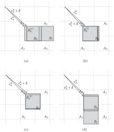
Figure6: Overlap property of MC block predicted by +δ, whereδ= {(1, 0), (−1, 0), (0, 1), (0,−1)}. (a) Overlap property ofB0predicted byv0

n+ (1, 0). (b) Overlap property ofB0predicted byvn0+ (−1, 0).

(c) Overlap property ofB0 predicted byvn0+ (0, 1). (d) Overlap

property ofB0predicted byvn0+ (0,−1).

2.4. Efficient method for extracting MC-DCT block in MVR

To apply the criterion function of (17), the motion com-pensated DCT macroblock with motion vector of (v0

n +δ)

is to be extracted from the reference frame. Let the MC-DCT macroblockMn(predicted byvn0ofΩn) be composed

of four blocks B0, B1, B2, and B3 according to relative locations (top left, top right, bottom left, bottom right), respectively. The extraction is to find the MC-DCT block from the intersecting blocks Ai (i = 0, 1, 2, 3) pointed by

a motion vector (MV) in the reference frame fk−1. One possible solution is illustrated in (11). However, it is too heavy for real-time application.

The work in [9] exploited the overlapping property of consecutive prediction. As shown in Figure 6(a), the MC-DCT block, predicted byv0

n+ (1, 0), is displaced fromB0by one pixel in the right. The superscript “r” inB0rdenotes the right displacement by one pixel. (Similarly, the superscripts “l,” “u,” and “d” denote the left, upward, and downward displacement by one pixel, resp.) Thus,Br

0overlapsB0by 8

×7 pixels andB1by 8×1 pixels (Figure 6(a)). To extractBr0, (13) is proposed, where

R=

0 0 I7 0

, S=

0 I1 0 0

. (12)

Ikis an identity matrix with sizek×k:

Wr=

0 Tmx

0 0

,

Br0=B0R+B1S,

Br

1=B1R+

i=1,3

PiAiWr,

Br2=B2R+B3S,

Br3=B3R+

j=1,3

PjAjWr.

(13)

For the caseBl0predicted byvn0+ (−1, 0),Bl0overlapsB0by 8

×7 pixels and partially overlapsA0andA2(Figure 6(b)). To extractBl

0, [9] proposes (14), whereRT is DCT(RT),

Wl=

0 0

U8−mx 0

,

Bl0=B0RT+

i=0,2

PiAiWl,

Bl1=B1RT+B0ST,

Bl2=B2RT+

j=0,2

PjAjWl,

Bl3=B3RT+B2ST.

(14)

Ukis a matrix with sizek×k, where only (0, 0)th component

is 1 with others being zero. Similarly, [9] propose (15) and (16) to extractBu

0(predicted byvn0+(0, 1)) andBd0(predicted byv0

n+ (0,−1)), respectively,

Wu=

0 U8−my

0 0

,

B0u=RB0+

i=0,1

WuAiQi,

Bu1=RB1+

j=0,1

WuAjQj,

B2u=RB2+SB0,

B3u=RB3+SB1,

(15)

Wd =

0 0

Tmy 0

,

Bd

0 =RTB0+STB2,

Bd

1 =RTB1+STB3,

Bd2=RTB2+

i=2,3

WdAiQi,

Bd3=RTB3+

j=2,3

WdAjQj.

(16)

For the caseB1dir, where dir∈ {r,l,u,d}, a similar algorithm is applied to extract the DCT block predicted byv0

(6)

(−2,−2) C0 2

C0 1

C00

(−2, 2)

C1 2

C1 1

C00

(2, 2) (2, 2)

LMV

BMV

Figure7: Fast searching pattern using LMV.

B1 B2

Downsizing

B3 B4 B

?

MV3 (0,−5) MV4 (−1,−1)

MV1 (1,−1)

(0, 5) MV2 Input motion vector Output motion vector

Figure8: Example of the diﬀerent direction motion vectors having the same value.

the overlap information. If the four intersected blocks are denoted asAi (i ∈ {0, 1, 2, 3}), the required equations for

extracting the desired DCT block are the second equations of (13), (14), (15), and (16).Tk is a matrix with sizek×k,

where only (k−1,k−1)th component is one and other components are zero. For the case of Bdir2 , where dir ∈

{r,l,u,d}, the third equations are applied. For the case of

Bdir3 , where dir∈ {r,l,u,d}, the fourth equations are applied. For the case ofBidir, wherei∈ {1, 2, 3}and dir∈ {r,l,u,d},

if the displaced block is fully overlapped with previously obtained MC-DCT blocks, the form of the equation is like the first equations of (13) and (16). However, if the displaced block is partially overlapped with the intersected blocksAi,

the equation form will be like the first equations of (14) and (15). Therefore, to extract a DCT macroblock displaced by one pixel in any direction from the previously obtained DCT macroblock, the required computation is largely reduced.

2.5. DCT-domain block matching criterion

From energy conservation property, the signal energy in the DCT-domain is equal to the energy in the pixel-domain. The base motion vector results in local motion variation in current macroblock. In order to eﬃciently capture the variation, we define a localized search area. Since the base motion vectorv0

n is available, block matching between the

(k−1)th frame (fk−1) and thekth frame (fk) amounts to

find the refinement vector δn for each target Ωn by MSE.

However, DCT-domain MSE is defined by:

δn=arg ⎛ ⎜ ⎝min

δ∈SL ⎛ ⎜ ⎝

p∈Ωn

fk(p)−fk−1(p+vn0+δ)

2

⎞ ⎟ ⎠ ⎞ ⎟ ⎠,

(17)

where fkis the DCT-domain version ofkth frame fk,Ωnis

thenth DCT macroblock in fk,vn0is the base motion vector

ofΩn,pis the position vector,δis the delta vector, andSL

is the local search area (LSA) depending on original motion vectors. The refined motion vector forΩnis defined by:

vn=vn0+δn. (18)

As the nonzero DCT coeﬃcients statistically concentrate on the neighborhood of DC component, only few coeﬃcients are considered in the new criterion. This will alleviate the burden in DCT matching.

2.6. Fast search (FS) algorithm

Seo and Kim [9] proposed that base motion vector from the median method is good enough to achieve the small search window (−2, +2). However, it is still not suitable for the MVR in the DCT-domain. Thus, it is highly desired to reduce the search area as much as possible. For this purpose, [9] introduces a localization motion vector (LMV). The LMV is detected by calculating the average of three motion vectors except the base one. Figure 7 shows an example of the proposed fast search algorithm. In this example, the LMV points at (1,−2). The shaded area is called the localized search area, which corresponds toSLin (17). The

checkpoints in the localized search area are considered for MVR.

(7)

Pixel Pixel

Integral point Half point Target point

(b) (a)

Figure9: (a) MVxand MVyare all nonintegral (b) MVxorMVyis nonintegral.

VLC

IQ2

+ FM MC-DCT2

Q2

−

DCT domain down-conversion

Refine MV MVs _resamplingMotion

(HFMR) FM

MC-DCT1 +

IQ1 VLD

CIF QCIF

Figure10: Using FRNI in CDDT.

Start

HFMR

Yes Use (20) to choose

a motion vector

More than one

MV is chosen? Use (21) to decideone vector No

No

Non-integral MV? Yes FRNI

FRNI

End

Figure11: Flow chart of the entire proposed HFMR and FRNI.

can apply refinement with fewer point (compared with traditional refinement), it is thereby referred to as fast search (FS).

3. PROPOSED ARCHITECTURES

It is obvious that three problems occurred in DCT-domain video transcoding.

(1) It is elaborate to extract macroblock in DCT-domain. (2) It is diﬃcult to refine motion vector in DCT-domain. Therefore, transcoding in DCT-domain needs more accurate motion vector than pixel domain.

(3) However, nonrefined motion vector is not suitable for video transcoder in DCT-domain.

In order to solve these problems, we propose the following algorithms.

3.1. Hierarchical fast motion resampling (HFMR)

Fast motion resampling (FMR) is always performed by simple operations (such as average, median filtering, and weighting) to reduce computation complexity and get new motion vector. It is based on the property of motion vectors and macroblock activity. Among those operations, median filtering can reach general performance for all sequences as in:

v= 1

2argvi∈{vmin1,v2,v3,v4}

4

j=1,j /=i

vi−vj. (19)

(8)

VLC

IQ2

+ FM MC-DCT2

Q2

−

DCT domain down-conversion

MVR MVs Motion

resampling (HFMR) FM

MC-DCT1 +

IQ1 VLD

CIF QCIF

Figure12: The architecture of CDDT with MVR.

1/8 1/4 1/2 1 2

βvalue 0.38

0.4 0.42 0.44 0.46 0.48 0.5

Ratio

Figure13:βand ratio.

motion vectors have the same value under usual circum-stances. For example, considering four motion vectors: (1,−1), (0, 5), (−1,−1), and (0,−5), both motion vectors (1,−1) and (−1,−1) have the minimum value as shown in

Figure 8. Therefore, we must further evaluate two motion vectors.

The number of nonzero coefficient is related to the residue energy. When fewer nonzero DCT coefficients are presented, less residue energy indicates that the predicted motion vector is more accurate. According to the observa-tion, the number of nonzero DCT coefficients is applied to decide motion vector in this situation. As in (20), we choose MV by minimum value of Av j. However, v j is detected

by (19), and all v j are of the equivalent minimum value. Av j denotes the number of nonzero DCT coeﬃcients in

macroblock and detected byv j:

v=1

2argvj∈{vmin1,v2,v3,v4}

Av j. (20)

3.2. Fast refinement for nonintegral MV (FRNI)

As mentioned above, nonrefined motion vector is not suitable for video transcoder in DCT-domain. However, it is diﬃcult to refine motion vector in DCT-domain. In MC-DCT, we have to extract more than one block for nonintegral

Start

i(an index)=0

DRSP

Yes

αi<

Q2

Q1

1/4

×αf

No

No Check cross-points

i=i+ one

Yes Is center point

minimum?

Detect extended search point by small-Viand small-Hi

where “i” is the defined index

Yes iis equal to one ? No Check half-pixel DCSA

End

Figure14: Flow chart of the proposed DRS.

motion vector which generated from FMR. As shown in

Figure 9, we must extract all blocks of integral point to compose the block of target points which are detected by motion vector. Unfortunately, this motion vector generated by FMR is not always accurate enough.

(9)

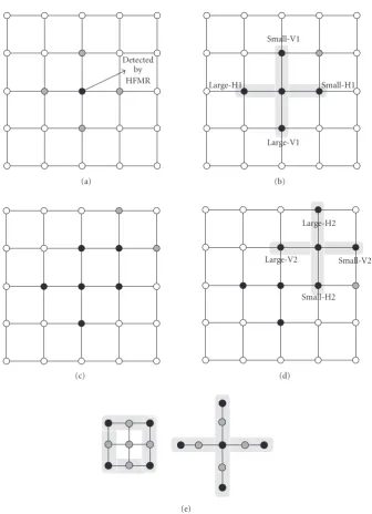
Detected by HFMR

(a)

Small-H1 Large-H1

Small-V1

Large-V1

(b)

(c)

Small-V2 Large-V2

Small-H2 Large-H2

(d)

(e)

Figure15: Steps in double cross-search algorithm: (a)Step 1, (b)Step 2, (c)Step 3, (d)Step 4, (e)Step 5of double cross-search algorithm.

reuse in [9] and the approach is from the fact that the basic motion vector decision, as called resampling, is diﬀ er-ent.

Due to this concept, we can get more useful data from MC-DCT without paying any additional operation. Fur-thermore, the proposed algorithm is easily combined with conventional architecture to get a more eﬃcient architecture. Based on our analysis, the computational complexity of extracted DCT block is larger than the criterion function. Therefore, it is essential to utilize the extracted blocks eﬃciently. As shown in Figure 9, we realize that there are nine additional checkpoints if MVx and MVy are all

nonintegral inFigure 9(a), and three additional checkpoints if MVx or MVy is nonintegral in Figure 9(b). Because

the blocks of integral points have been extracted, we can

obtain the additional checkpoints directly or by computing the average from extracted blocks. The black point in

Figure 9is decided by rounding nonintegral motion vector. Afterward, we use the absolute sum of DCT coefficients to determine the refined motion vector in (21), where MVoffset is the offset motion vector, S is the checkpoint detected by original motion vector, δ is the current checkpoint, MBδ is the residue block detected by δ, a is the

refine-ment motion vector distance, and MBδ−a is the extracted

block from DCT-domain with refined motion vector. The refined MV is defined as MVRefined = MVnon-refined + MVoﬀset:

MVoﬀset=arg min

δ∈S

3

a=0 63

i=0

(10)

40 60 80 100 120 140 160 180 200 Bit-rate (kbit/s)

26 26.5 27 27.5 28 28.5 29 29.5 30

PSNR

(dB)

HFMR-BR versus HFMR-PSNR Median-BR versus median-PSNR ACT-BR versus ACT-PSNR Average-BR versus average-PSNR WLF-BR versus WLF-PSNR

(a)

40 60 80 100 120 140 160 180 200 Bit-rate (kbit/s)

28 28.5 29 29.5 30 30.5 31

PSNR

(dB)

(b)

40 60 80 100 120 140 160 180 200 Bit-rate (kbit/s)

24.5 25 25.5 26 26.5 27 27.5

PSNR

(dB)

(c)

100 150 200 250 300 350 400 450 Bit-rate (kbit/s)

27 27.5 28 28.5 29 29.5 30 30.5 31

Y

data

(d)

Figure16: The R-D curves for diﬀerent FMR algorithm. (a) Foreman. (b) TableTennis. (c) Coastguard. (d) Football.

By using FRNI, we can get three advantages.

(1) Considering the rate distortion, we can obtain more suitable motion vector.

(2) FRNI does not increase the computation complexity for extracting MBs in DCT-domain.

(3) MV refinement can be separated into integer and half-pixel process. Since half-pixel refinement can be achieved by the integer search with some additions and decisions (based on the definition of FRNI), the complexity on MC-DCT can be reduced. This is obvious in DCT-domain since the compensation and prediction cannot be preformed directly from simple arithmetic.

The flow chart of the entire proposed algorithm is shown in Figure 11. It is constructed by two individual parts. For HFMR, it provides more accurate motion vector. In FRNI, we can get more suitable refined motion vector and reduce complexity of nonintegral motion vector in MC-DCT. Furthermore, the flow chart of the entire proposed algorithm is only performed in luminance component. As chrominance components, the coded type is decided based on its corresponding luminance component.

3.3. Dynamic regulating search (DRS)

(11)

20 40 60 80 100 120 140 160 Bit-rate (kbit/s)

26 26.5 27 27.5 28 28.5 29 29.5 30

PSNR

(dB)

Full search-BR versus full search-PSNR HFMR + FRNI-BR versus HFMR + FRNI-PSNR HFMR-BR versus HFMR-PSNR

(a)

40 60 80 100 120 140 160

Bit-rate (kbit/s) 28

28.5 29 29.5 30 30.5 31 31.5

PSNR

(dB)

(b)

20 40 60 80 100 120 140 160 180 200 Bit-rate (kbit/s)

24.5 25 25.5 26 26.5 27 27.5 28

PSNR

(dB)

(c)

100 150 200 250 300 350 400 450 Bit-rate (kbit/s)

27 28 29 30 31 32

PSNR

(dB)

(d)

Figure17: The R-D curves for our proposed FRNI. (a) Foreman. (b) TableTennis. (c) Coastguard. (d) Football.

are the same, since the search range is only decided by four input motion vectors. In video coding technique, quantization error dominates video coding distortions in low bit-stream saturation. Therefore, it is essential to reduce search points dynamically in low bit-rate. Furthermore, we also propose a novel fast MVR algorithm, double cross-search algorithm (DCSA), to improve the performance of MVR. The proposed algorithms are based on the architec-ture, as shown inFigure 12.

3.3.1. Dynamic reduced search points in MVR (DRSP)

Most of the refinement algorithms try to reduce computa-tional complexity by search range reduction or fast search algorithm. However, there are still heavy computational complexities since all the motion vectors in the frame are re-estimated in the refinement process. Therefore, we utilize the variance ofα and (Q2/Q1)β ×αf to be a criterion. αi

is the absolute sum of DCT coeﬃcients of current block and αf is the average value of blocks of previous frame.

Q1 is the quantization parameter of input stream and Q2 is the quantization parameter of output stream. β is a parameter for refinement threshold definition. To investigate the eﬀect of variousβon refinement points, an experiment is conducted with 5 patterns (1/8, 1/4, 1/2, 1, 2) forβand the result is presented inFigure 13. The experiment is performed on various sequences (including Foreman, Costguard, and TableTennis). Since the objective is to minimize refinement point, a criterion function is defined by:

ratio=(refined points)β=0−(refined points)β

(search point)_β₌₀−(search point)_β . (22)

(12)

20 40 60 80 100 120 140 160 Bit-rate (kbit/s)

26 26.5 27 27.5 28 28.5 29 29.5 30

PSNR

(dB)

Full search-BR versus full search-PSNR DRS-BR versus DRS-PSNR

FS[9]-BR versus FS[9]-PSNR HFMR-BR versus HFMR-PSNR

HFMR + FRNI-BR versus HFMR + FRNI-PSNR (a)

Qvalue 80

100 120 140 160 180 200 220 240 260 280

Sear

ch

points

FS[9] DRS

(b)

40 60 80 100 120 140 160

Bit-rate (kbit/s) 28

28.5 29 29.5 30 30.5 31 31.5

PSNR

(dB)

HFMR + FRNI-BR versus HFMR + FRNI-PSNR (c)

Qvalue 130

140 150 160 170 180 190 200 210

Sear

ch

points

FS[9] DRS

(d)

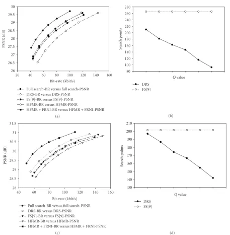
Figure18: Simulation results for DRS. (a) The R-D curves of Foreman. (b) Average search points per frame for Foreman. (c) The R-D curves of TableTennis. (d) Average search points per frame for TableTennis.

implemented to fulfill the goal in search point reduction:

if

αi< _Q

1 Q2

β ×αf

, then Non-refinement,

else, Refinement.

(23)

3.3.2. Double cross-search algorithm

After DRSP, we perform double cross-search algorithm for refined blocks. Overall flowchart is presented in Figure 14. When the criterion is matched in DRSP, double cross-search is performed. Initial search is performed on a “cross-like” area, and the shape is demonstrated inFigure 15(a). At the same time, an index “i” is defined and set to one. The index

is to number the iteration. If cost function is minimal at the center, refinement is stopped. Else, the search point is expended by the cross shape based on smaller horizontal and vertical motion vector, defined as H1 and small-V1. The refinement process repeated if the extension is performed. Since the loop is terminated when index “i” is equal or larger than 2, maximum iteration number is 2.

The following is an example for the proposed algorithm. Step 1. We use (21) to check the 4-neighboring points (up, down, left, and right). If the checkpoints are smaller than the center point, we expand search point in Step 2; otherwise, stop the search (Step 5). The process is shown in

(13)

20 40 60 80 100 120 140 160 180 200 Bit-rate (kbit/s)

24.5 25 25.5 26 26.5 27 27.5 28

PSNR

(dB)

HFMR + FRNI-BR versus HFMR + FRNI-PSNR (a)

10 12 14 16 20 25

Qvalue

227.7347

60 80 100 120 140 160 180 200 220 240

Sear

ch

points

FS[9] DRS

(b)

100 150 200 250 300 350 400 450 Bit-rate (kbit/s)

27 28 29 30 31

PSNR

(dB)

HFMR + FRNI-BR versus HFMR + FRNI-PSNR (c)

8 10 12 14 16 18 20 22 24 26

Xdata 100

150 200 250 300 350 400

Y

data

FS[9] DRS

(d)

Figure19: Simulation results for DRS. (a) The R-D curves of Coastguard. (b) Average search points per frame for Coastguard. (c) The R-D curves of Football. (d) Average search points per frame for Football.

Step 2. The expanded point is decided by Small-V1 and Small-H1. If the expanded point is smaller than Small-V1 and Small-H1, we expand search points in Step 3 further; otherwise, stop the search (Step 5). The process is as shown inFigure 15(b).

Step 3. As shown in Figure 15(c), we expand horizontal and vertical search points. If the prediction error of any checkpoint is smaller than the center one, we expand search point inStep 4; otherwise, stop search (Step 5).

Step 4. The expanded point is decided by Small-V2 and Small-H2, as shown inFigure 15(d).

Step 5. We perform search in half-pixel according to final search point. As shown inFigure 15(e), there are two possible patterns.

In addition to improving the efficiency of search, the proposed DRS has several advantages. First, we can control search range in (−2, 2) efficiently inStep 2. Second, we can search half-pixel points efficiently. Finally, we can reduce complexity further by combining with the efficient method in [9] for block extracting.

3.4. Overall design

(14)

Table3: Experimental results for three simulated sequences at QP=10.

Sequence name FMR Bitrate PSNR

Foreman

HFMR 143.12 29.6063

Median 146.31 29.5446

ACT-weighted 146.95 29.5928

Average 164.38 29.4295

WLF 178.17 29.3728

TableTennis

HFMR 149.55 30.822

Median 155.63 30.8285

Average 186.92 30.668

WLF 185 30.6177

Coastguard

HFMR 176.09 27.1596

Median 176.41 27.1623

Average 176.42 27.0714

WLF 192.57 26.8894

Table4: Reduced ratio of nonintegral in MC-DCT.

Sequence name Number of extracted DCT blocks for nonintegral MV (4 luminance blocks and 2 chrominance blocks) Reduced ratio

Nonrefined Refined

Foreman 4×6544 + 2×9114 4×6544 + 2×7220 8.50%

Table 4×6560 + 2×8976 4×6560 + 2×6696 11.30%

Coastguard 4×6100 + 2×7904 4×6100 + 2×6738 5.8%

quality than nonrefine motion vector and reduce the com-plexity. DRS can utilize the filter for half-pixel motion vector in MC-DCT [8] and eﬃcient method for extracting MC-DCT block [9] to improve the performance.

4. EXPERIMENTAL RESULTS

4.1. Experiment environment

We simulate the proposed algorithms in software by

transcoding H.263 CIF (352 × 288) bit streams to QCIF

(176 by 144). The simulated four well-known sequences areForeman,Coastguard,TableTennis, andFootball.Foreman andTableTennisis with median motion activity.Costguard is with low motion activity. Football is with high motion activity. Since the performance is deeply related with motion activity, the sequences can show the performance under various circumstances. In order to get better comparison with the other methods, the coding style of each input stream is IPPPPPP with 50 frames and 30 frames/s. The test sequences are first encoded at quantization parameter (QP) of 6. Afterward, six transcoders (with QP=10, 12, 14, 16, 20, and 25) are applied for transcoding, respectively. The full search range is (−2, 2).

4.2. Experiment result of HFMR

We compare with the other FMR algorithms, ACT-weight, median filter, average, and WLF-max. The rate-distortion (R-D) curves of test sequences,Foreman,TableTennis,Costguard, andFootball, are shown in Figures16(a),16(b), 16(c), and

16(d), respectively. In Table 3, we also show the average

PSNR and bit-rate at QP = 10 for three sequences. The

objective of HFMR is to ensure consistent quality among various video sequences. Thus, slight modification is made on conventional approaches. According to the experimental results, HFMR is with highest quality among all. The reason for similar performance is from the fact that resampling applies simple method to obtain a rough motion vector. Since it is not refined extensively, the eﬀect on performance is limited.

4.3. Experiment result of FRNI

In this subsection, we show the experiment results of FRNI for the test sequences. It is quite clear that the performance for all test sequences (Foreman, TableTennis, Coastguard, and Football) is improved at various QPs after combining with FRNI shown in Figures17(a),17(b),17(c), and17(d), respectively.

InTable 4, we show the total numbers of extracted DCT blocks for half-pixel motion vectors and the reduced ratios. The results prove that the proposed FRNI will not induce extra computational complexity in MC-DCT. However, it can get about 8.5% of reduction with the proposed HFMR in average. Note that the reduced operation of extracted block is larger than the checked point.

4.4. Experiment result of DRS

(15)

search points between [9] and DRS are shown in Figures18, and19(b), and19(d). Quantization parameters for (a)–(c) and (b)–(d) are the same, as illustrated in (b)–(d). For the best case (TableTennis) DRS can improve performance and reduce search points in all diﬀerent QPs. The reduction of search points is about 29%, especially at QP of 25. As to the normal cases, we do not only preserve the quality but also

reduce 21% ∼ 65% and 12% ∼ 69% of search points for

FormanandCoastguard, respectively. The only exception falls in the sequenceFootball. However, the performance of DRS is obviously higher than FS. From the results, proposed DRS can achieve higher performance (compared with FS) while the search point is reduced in average. When the search point is higher, performance of DRS is relatively strong compared with other algorithms.

The search point for HFMR-FRNI is smaller than DRS. However, the performance in DRS is better than

HFMR-FRNI. Since it is a tradeoﬀ between search point and

performance, the adoption of specific approach is considered based on the given constraint. If faster approach is desired, HFMR-FRNI is a better choice. If better performance is desired, DRS is the best candidate.

5. CONCLUSION

This article presented several techniques for spatial resolu-tion reducresolu-tion for video transcoder in DCT-domain. For motion vector resampling, our proposed HFMR modified the median filter to improve the entire quality further.

As to MVR, we proposed FRNI and DRS for diﬀerent

architectures. FRNI is based on brute-force MC-DCT to only refine half-pixel motion vector. DRS reduced search points dynamically and achieved eﬃcient refinement by DRSP and DCSA, respectively.

From the experiments, we believe that the proposed HFMR outperforms the other techniques for all simulated sequences. Besides, two MVR algorithms also improved the entire quality eﬃciently, especially DRS. For the best case, DRS can improve performance and reduce search points in all diﬀerent QPs. Compared with [9], the reduction of search points is about 29%. As to the normal cases, it does not only preserved the quality but also reduced 16%∼67% of search points.

REFERENCES

[1] A. Vetro, C. Christopoulos, and H. Sun, “Video transcoding architectures and techniques: an overview,”IEEE Signal Pro-cessing Magazine, vol. 20, no. 2, pp. 18–29, 2003.

[2] P. Yin, A. Vetro, B. Liu, and H. Sun, “Drift compensation for reduced spatial resolution transcoding,”IEEE Transactions on Circuits and Systems for Video Technology, vol. 12, no. 11, pp. 1009–1020, 2002.

[3] W. Zhu, K. H. Yang, and M. J. Beacken, “CIF-to-QCIF video bitstream down-conversion in the DCT domain,”Bell Labs Technical Journal, vol. 3, no. 3, pp. 21–29, 1998.

[4] B. Shen, I. K. Sethi, and B. Vasudev, “Adaptive motion-vector resampling for compressed video downscaling,”IEEE Transactions on Circuits and Systems for Video Technology, vol. 9, no. 6, pp. 929–936, 1999.

[5] K.-T. Fung and W.-C. Siu, “DCT-based video downscaling transcoder using split and merge technique,”IEEE Transac-tions on Image Processing, vol. 15, no. 2, pp. 394–403, 2006. [6] Y.-R. Lee and C.-W. Lin, “DCT-domain spatial transcoding

using generalized DCT decimation,” in Proceedings of IEEE International Conference on Image Processing (ICIP ’05), vol. 1, pp. 821–824, Genova, Italy, September 2005.

[7] Y.-R. Lee and C.-W. Lin, “Visual quality enhancement in DCT-domain spatial downscaling transcoding using generalized DCT decimation,”IEEE Transactions on Circuits and Systems for Video Technology, vol. 17, no. 8, pp. 1079–1084, 2007. [8] G. Cao, Z. Lei, J. Li, N. D. Georganas, and Z. Zhu, “A novel

DCT domain transcoder for transcoding video streams with half-pixel motion vectors,”Real-Time Imaging, vol. 10, no. 5, pp. 331–337, 2004.

[9] K.-D. Seo and J.-K. Kim, “Fast motion vector re-estimation for transcoding MPEG-1 into MPEG-4 with lower spatial resolution in DCT-domain,”Signal Processing: Image Commu-nication, vol. 19, no. 4, pp. 299–312, 2004.

[10] S.-F. Chang and D. G. Messerschmitt, “A new approach to decoding and compositing motion-compensated DCT-based images,” in Proceedings of IEEE International Conference on Acoustics, Speech and Signal Processing (ICASSP ’93), vol. 5, pp. 421–424, Minneapolis, Minn, USA, April 1993.

[11] N. Merhav and V. Bhaskaran, “Fast algorithms for DCT-domain image downsampling and for inverse motion com-pensation,”IEEE Transactions on Circuits and Systems for Video Technology, vol. 7, no. 3, pp. 468–476, 1997.

[12] N. Merhav, “Multiplication-free approximate algorithms for compressed-domain linear operations on images,” IEEE Transactions on Image Processing, vol. 8, no. 2, pp. 247–254, 1999.

[13] K. N. Ngan, D. Chai, and A. Millin, “Very low bit rate video coding using H.263 coder,”IEEE Transactions on Circuits and Systems for Video Technology, vol. 6, no. 3, pp. 308–312, 1996. [14] Y.-R. Lee, C.-W. Lin, and C.-C. Kao, “A DCT-domain video

transcoder for spatial resolution downconversion,” in Proceed-ings of the 5th International Conference on Recent Advances in Visual Information Systems (VISUAL ’02), vol. 2314 ofLecture Notes in Computer Science, pp. 207–218, Hsin Chu, Taiwan, March 2002.