Bingo at IJCNLP-2017 Task 4: Augmenting Data using Machine
Translation for Cross-linguistic Customer Feedback Classification
Heba Elfardy, Manisha Srivastava, Wei Xiao, Jared Kramer, Tarun Agarwal {helfardy,mansri,weixiaow,jaredkra,tagar}@amazon.com
Amazon Seattle, WA, USA
Abstract
The ability to automatically and accurately process customer feedback is a necessity in the private sector. Unfortunately, cus-tomer feedback can be one of the most difficult types of data to work with due to the sheer volume and variety of ser-vices, products, languages, and cultures that comprise the customer experience. In order to address this issue, our team built a suite of classifiers trained on a four-language, multi-label corpus released as part of the shared task on “Customer Feed-back Analysis” at IJCNLP 2017. In ad-dition to standard text preprocessing, we translated each dataset into each other lan-guage to increase the size of the training datasets. Additionally, we also used word embeddings in our feature engineering step. Ultimately, we trained classifiers us-ing Logistic Regression, Random Forest, and Long Short-Term Memory (LSTM) Recurrent Neural Networks. Overall, we achieved a Macro-Average Fβ=1score be-tween 48.7% and 56.0% for the four lan-guages and ranked 3/12 for English, 3/7 for Spanish, 1/8 for French, and 2/7 for Japanese.
1 Introduction
Customer feedback constitutes the primary back-channel for improving most business offerings. Due to the sheer volume that is typical for cus-tomer feedback, there is a strong industry need for systems that can automatically classify this data. Unfortunately, this classification task is not straightforward; every product has a unique customer experience and every company has particular goals when extracting constructive
information from feedback. These targets vary across not only products and services, but across the languages and cultures of their customers as well. To complicate the matter further, the private nature of businesses in need of this classification–as well as businesses offering this classification as a service–has resulted in a lack of any agreed-upon classification standards.
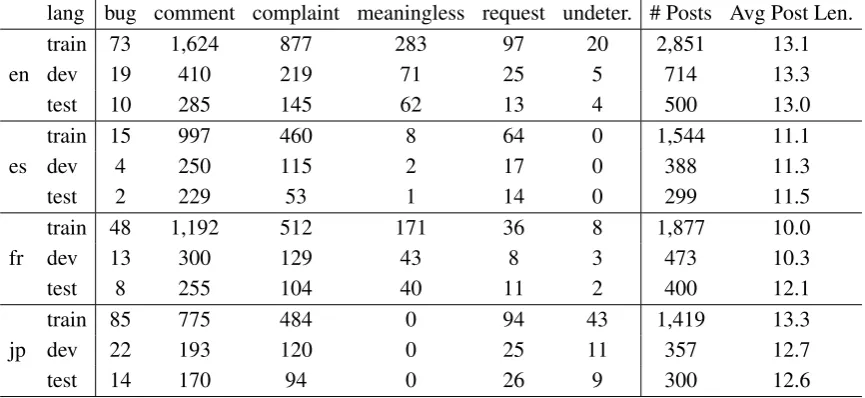
To address this gap, IJCNLP 2017 hosted a shared task and released a corpus of multi-lingual, multi-label customer feedback. This data is orga-nized according to a five-plus-one label schema consisting of the following labels: “bug”, “com-ment”, “complaint”, “meaningless”, “request” or “undetermined” across four languages; English (en), Spanish (es), French (fr) and Japanese (jp). As part of this shared task, our team has trained a suite of classifiers over this corpus and here reports the performance of our system. In the remainder of this paper, we will first describe related work in Section 2 before briefly describ-ing the dataset in Section 3. In Section 4, we describe our classification approach, including the translation of the data, our approach to feature engineering, and the learning methods used to train our classifiers, before offering results and discussion in Section5.
2 Related Work
While text classification is a well-established field, its application on customer feedback is somewhat less mature. One area that has received a fair amount of attention is the task of sentiment classification of customer feedback (Gupta et al.,
2010; Gamon, 2004; Kiritchenko et al., 2014). However, sentiment classification enjoys the use of established labeling schemas, typically two, three, or five-way labeling to indicate the presence
lang bug comment complaint meaningless request undeter. # Posts Avg Post Len.
train 73 1,624 877 283 97 20 2,851 13.1
en dev 19 410 219 71 25 5 714 13.3
test 10 285 145 62 13 4 500 13.0
train 15 997 460 8 64 0 1,544 11.1
es dev 4 250 115 2 17 0 388 11.3
test 2 229 53 1 14 0 299 11.5
train 48 1,192 512 171 36 8 1,877 10.0
fr dev 13 300 129 43 8 3 473 10.3
test 8 255 104 40 11 2 400 12.1
train 85 775 484 0 94 43 1,419 13.3
jp dev 22 193 120 0 25 11 357 12.7
test 14 170 94 0 26 9 300 12.6
Table 1: Number of posts per class and average post length in the training (folds 1-4), development (fold 5) and held-out test sets of the dataset
or intensity of positivity, negativity, or neutrality of customer text (Balahur et al.,2014).
More recently, several customer feedback la-beling schemas have been published, including
Bentley and Batra (2016) who make the dis-tinction between Customer Service data and Customer Feedback such as product reviews and in-app comments. The authors classify text according to product-specific labels defined by domain experts. Potharaju et al. (2013) built a system to identify three distinct labels in network trouble tickets including problem symptoms, troubleshooting activities and resolution actions.
Arora et al. (2009) classify product reviews as qualified claims or bald claims depending on how quantifiable a customer claim is. Other labeling schema do of course exist, though they are kept private as part of private products that help users analyze and synthesize customer complaints and comments.
3 Data
In an effort to close the gap in a unified labeling schema for customer feedback, this shared task on Customer Feedback Analysis aims to organize customer feedback according to a more univer-sally applicable label set. This label set includes: “bug”, “comment”, “complaint”, “meaningless”, “request” or “undetermined”. This label set is multi-label where each customer utterance can belong to one or more of these classes. For example, “We didn’t eat there again and thankful
it was only 1 night.” is both a “comment” and a “complaint” while “Transactions made on week-end are updated on Tuesday Please improve.” is a “request” and a “complaint”. The corpus that was created for this shared task consists of data for four languages: English (en), Spanish (es), French (fr), and Japanese (jp).
Language Without Translations With Translations Percentage Increase
en 3,565 9,623 170%
es 1,932 9,623 390%
fr 2,350 9,623 309%
jp 1,776 9,623 442%
Table 2: Number of utterances in the training data before and after including the translations from all other three languages
performance. For the development set, we tune our systems using the unweighted average Fβ=1 score of all six class labels. However, on the test set we also report Micro and Macro averages.
4 Approach
We train classifiers using three different learning methods: Random Forest, Logistic Regression, and Long Short-Term Memory Recurrent Neural Network (LSTM). In this section, we describe our data preprocessing (including machine translation of the sub-corpora), our use of word embedddings, and each of the learning methods used to train our classifiers.
4.1 Preprocessing
We tokenize and stem the English and Spanish data using Stanford Core NLP toolkit (Manning et al., 2014) . For French, we use an in-house tool for both tokenization and stemming while for Japanese, we use MeCab (Kudo,2005) to tokenize the data.
4.2 Translation
We translate the data in each language pairwise to the other three languages to increase the size of the training data. Our assumption here was that the increased amount of data would more than make up for the introduction of noise that comes from using machine translation. We use the Neural Machine Translation (NMT) model in Google Cloud Translation API 1 to perform the
translations.
Table 2 shows the number of labeled sen-tences that were provided in each language, and the number of labeled sentences after translation.
1https://cloud.google.com/translate/ docs
4.3 Word Embeddings
Word-embeddings convert the high-dimensional n-grams space to a low-dimensional continuous vector space by calculating the distributional sim-ilarity of words. Accordingly, words that tend to occur in similar contexts will be close to each other in the resulting vector space. Word-embeddings have been shown to help with a vari-ety of NLP tasks (Socher et al.,2011;Turian et al.,
2010;Collobert et al.,2011;Baroni et al.,2014). For each language, we use Facebook’s FastText embeddings (Bojanowski et al., 2016) that were trained on that language’s Wikipedia articles to generate a vector of 300 dimensions for each word in a given tokenized utterance. As opposed to Word2Vec (Mikolov et al., 2013) which assigns a vector to each word, FastText represents each word as a bag of character n-grams and maps each character n-gram to a vector. Accordingly, it is able to model the morphology of words.
4.4 Learning Methods
We train classifiers using three learning methods: Random Forest, Logistic Regression, and LSTM. In this section, we provide a brief overview of each learning method.
4.4.1 Random Forest
(Friedman et al.,2001).
4.4.2 Logistic Regression
For our Logistic Regression classifier we use the implementation included in the Scikit-Learn toolkit (Pedregosa et al.,2011)2. Logistic
Regres-sion is a regresRegres-sion model for classification prob-lems where a logistic function is used to model the probabilities of all possible class labels of a data instance. We use L2 regularization and set the in-verse of regularization strength (C) to 100.
4.4.3 LSTM
We also experiment with an LSTM classifier. A sentence is a sequence of words, and LSTM is a now common approach for sequence classifica-tion. It encodes an entire sentence into a feature vector which is used to classify the sentence instead of using bigrams/trigrams occurring in the sentence. LSTMs use the embeddings of the words, hence encode the semantic similarity be-tween words that occur in similar contexts. Using embeddings also helps in reducing the sparsity problem that we encounter with bigrams/trigrams models.
For this classifier, we map each input sen-tence to a sequence of maximum length 30, and pad the sequence with zeros if the length is less than 30. We initialize the embedding using the pre-trained embeddings presented earlier in Section 4.3. Our final LSTM architecture has 80 nodes–except for French, where each LSTM has 100 nodes–and 0.1 dropout on both the input and hidden layer weights. Using the same hyper parameters for the French model resulted in a poor performance, so the number of nodes in the LSTM was increased to 100. The last layer is a fully-connected layer with six output nodes corresponding to the six output classes. We used RMSProp optimizer to train the model. For prediction, we create a one-hot-encoding for the output labels. For each multi-label utterance, we create two samples, one for each label. We use a sigmoid function at the final layer instead of softmax, in order to be able to threshold each output node individually to decide whether the input sentence belongs to that class or not.
2http://scikit-learn.org/ stable/modules/linear_model.html# logistic-regression
class en es fr jp
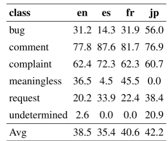
bug 31.2 14.3 31.9 56.0 comment 77.8 87.6 81.7 76.9 complaint 62.4 72.3 62.3 60.7 meaningless 36.5 4.5 45.5 0.0 request 20.2 33.9 22.4 38.4 undetermined 2.6 0.0 0.0 20.9 Avg 38.5 35.4 40.6 42.2
Table 3: Development Set Performance of Ran-dom Forest measured in Fβ=1score
class en es fr jp
bug 31.2 40.0 21.1 45.0 comment 79.7 88.6 81.8 81.4 complaint 60.4 61.4 58.2 57.7 meaningless 41.9 0.0 37.3 0.0 request 30.3 53.3 32.0 50.9 undetermined 0.0 0.0 0.0 20.0 Avg 40.6 40.6 38.4 42.5 Micro Avg 64.5 78.0 67.2 65.9 Macro Avg 42.5 50.0 39.7 52.3
Table 4: Held-Out Test Set Performance of Ran-dom Forest measured in Fβ=1score
Since the labels’ distribution in the training data is skewed, we weight the classes inversely by the number of utterances of the class in the training data. The weights assigned to the classes are as follows: “bug”: 20.0, “complaint”: 2.0, “comment”: 1.0, “meaningless”: 10.0, “request”: 20.0, “undetermined”: 50.0
We train a separate LSTM for each language. The vocabulary size for all four LSTMs is 7,000. All models are trained for 10 epochs with a learning rate of 0.001 and optimized using a categorical cross-entropy loss function.
5 Results & Discussion
en es fr jp
Ngram 37.5 34.8 33.8 43.4
Ngram-Stem 39.2 33.6 31.8
-Ngram+Stem 36.2 36.6 36.0
-EMB 32.0 29.1 36.3 30.5
Ngram+EMB 40.7 38.6 39.2 40.1
Ngram-Stem+EMB 40.2 41.9 34.3
-Ngram+Stem+EMB 41.6 39.2 36.2
-Table 5: Development Set Performance of different setups of Logistic Regression measured in Fβ=1 score
en es fr jp bug 40.0 22.3 21.1 57.9 comment 78.7 90.6 82.3 83.6 complaint 59.1 71.6 68.7 68.0 meaningless 38.5 16.7 43.8 0.0 request 33.3 50.0 15.4 41.9 undetermined 0.0 0.0 4.3 8.9 Avg 41.6 41.9 39.2 43.8
Table 6: Per-class Development Set Performance of Logistic Regression measured inFβ=1score
5.1 Random Forest
We use standard n-gram features (1 to 3) and pre-trained FastText word-embeddings to train a binary Random Forest classifier for each of the different classes. For word embeddings, we calculate the average of embeddings of all words in a given training/test instance and use the resulting scores as features. In this experiment, we do not augment each language’s training data with the translations and only rely on each language’s training data. Here we choose separate cutoff point for each class. The cutoff point for a class is defined in such a way that if the predicted probability is larger than the cutoff point, then the corresponding label is added to the prediction for the sentence. The cutoff point for a class is chosen by maximizing the average Fβ=1 score of the corresponding class over the five pairs of training and development datasets. The performance of Random Forest on the development and test sets is given in Tables3and4.
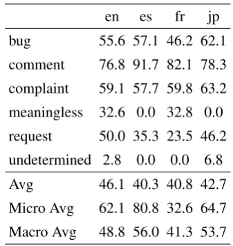
en es fr jp bug 55.6 57.1 46.2 62.1 comment 76.8 91.7 82.1 78.3 complaint 59.1 57.7 59.8 63.2 meaningless 32.6 0.0 32.8 0.0 request 50.0 35.3 23.5 46.2 undetermined 2.8 0.0 0.0 6.8 Avg 46.1 40.3 40.8 42.7 Micro Avg 62.1 80.8 32.6 64.7 Macro Avg 48.8 56.0 41.3 53.7
Table 7: Held-Out Test Set Performance of Lo-gistic Regression measured inFβ=1score
5.2 Logistic Regression
For this model, we experiment with the following feature sets for each language:
• N-grams: For this feature-set, we use the TFIDF score of n-grams (1 to 3) that ap-pear in more than five training instances. For Japanese data, we use the MeCab-tokenized text while for the other three languages we use the white-space tokenzied text.
• Stemmed N-grams: In addition to tradi-tional n-grams, we use the stemmed English, French and Spanish data to extract stemmed n-grams.
• Word Embeddings: Similar to the Random Forest experiment, we use the average of em-beddings of all words in a given training/test instance as features in our classifier.
for each language with the translations of the other three languages data into this language. As noted earlier, our assumption is that the increase in the size of each dataset would lead to improved performance despite the noisey nature of machine translation. This assumption was born out in that adding translated data resulted in 8.82% average Fβ=1 improvement on the English development dataset.
Table 5 shows the average Fβ=1 score for the different experimental setups. Table6 shows the Fβ=1 for each of the six classes for the best development setup for each language.
For English, Spanish and French, combining n-grams with word-embeddings yields best results. The only difference between each of the three languages is whether the best setup involves using basic n-grams, stemmed n-grams or both. For Japanese, adding word-embeddings degrades the performance. This could be due to a discrepancy in our tokenization scheme and the tokenization scheme used to train the embeddings’ model. The best performance is achieved on “comment” class since it is the most dominant class in the training data and the worst performance is on “undetermined” class since the percentage of training instances that have that class is almost negligible.
Table 7 shows the results using the best de-velopment setup on the held-out test set. Similar to the development set, the performance of each class directly correlates with how well it is represented in the training data.
5.3 LSTM
For all languages and all classes a threshold of 0.7 is used. The threshold was chosen to maximize the average Fβ=1score on the development set. If the sigmoid value of the output node is more than the threshold, the corresponding output label is added to the input sentence. If none of the output nodes crosses the threshold, the input sentence is labeled as “comment” which is the majority class in all languages.
Table 8 shows the Fβ=1 score of the model on the development set. The model performs sig-nificantly better on the Japanese data. Across all
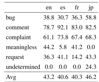
en es fr jp bug 38.8 30.7 36.3 58.8 comment 78.7 92.1 83.0 82.5 complaint 61.1 73.8 67.4 68.3 meaningless 44.2 5.8 41.2 0.0 request 36.3 41.1 14.2 43.3 undetermined 0.0 0.0 0.0 24.3 Avg 43.2 40.6 40.3 46.2
Table 8: Development Set performance of LSTM model measured in Fβ=1score
en es fr jp bug 45.1 21.0 28.5 48.0 comment 78.7 92.6 67.2 80.0 complaint 45.0 66.0 84.8 60.4 meaningless 45.7 0.0 49.1 0.0 request 27.1 52.0 34.7 44.7 undetermined 0.0 0.0 6.8 20.0 Avg 40.3 38.6 45.2 42.1 Micro Avg 60.8 78.2 69.7 64.1 Macro Avg 45.1 52.0 48.7 53.8
Table 9: Test Set performance of LSTM model measured in Fβ=1score
languages, and similar to the previous two models, the model performs best on the most dominant classes–“complaint” and “comment”. Also, the performance of the model on “meaningless” and “undetermined” classes is significantly worse because there is not enough training examples for the model to be able to distinguish these classes. Table 9 shows the performance of the model on the held-out test data. Similar to the development set, the model performs best on Japanese.
5.4 Ranking
on French and Japanese and ranked 1/8 and 2/7 on each of them while Logistic Regression performed best on English where it ranked 3/12 and Spanish ranking 3/7.
6 Conclusion
This shared task was created with the intent of es-tablishing a labeling schema that is both widely applicable and publicly available. Ultimately, the performance of our classifiers varied a fair amount with respect to the different metrics. Overall, us-ing Macro-Average Fβ=1, we ranked 3/12, 3/7, 1/8 and 2/7 on English, Spanish, French and Japanese datasets respectively. The inclusion of word embeddings and machine translation offered the largest boosts to system performance. Future directions for work in this area could include ex-panding the amount of data, which in turn might improve the performance of deep learning meth-ods. Included in this shared task was an unan-notated dataset for each language. Though our team did not explore a semi-supervised approach, our experiments with translated data indicate this would be low-hanging fruit.
References
Shilpa Arora, Mahesh Joshi, and Carolyn P Ros´e. 2009. Identifying types of claims in online customer re-views. InProceedings of the Annual Conference of the North American Chapter of the Association for Computational Linguistics.
Alexandra Balahur, Rada Mihalcea, and Andr´es Mon-toyo. 2014. Computational approaches to subjec-tivity and sentiment analysis: Present and envisaged methods and applications. Computer Speech & Lan-guage, 1(28):1–6.
Marco Baroni, Georgiana Dinu, and Germ´an Kruszewski. 2014. Don’t count, predict! a systematic comparison of context-counting vs. context-predicting semantic vectors. InProceedings of the 52nd Annual Meeting of the Association for Computational Linguistics.
Michael Bentley and Soumya Batra. 2016. Giving voice to office customers: Best practices in how of-fice handles verbatim text feedback. In2016 IEEE International Conference on Big Data, pages 3826– 3832. IEEE.
Piotr Bojanowski, Edouard Grave, Armand Joulin, and Tomas Mikolov. 2016. Enriching word vec-tors with subword information. arXiv preprint arXiv:1607.04606.
Leo Breiman. 2001. Random forests. Machine Learn-ing, 45(1):5–32.
Ronan Collobert, Jason Weston, L´eon Bottou, Michael Karlen, Koray Kavukcuoglu, and Pavel Kuksa. 2011. Natural language processing (almost) from scratch. Journal of Machine Learning Research, 12(Aug):2493–2537.
Jerome Friedman, Trevor Hastie, and Robert Tibshi-rani. 2001. The Elements of Statistical Learning, volume 1. Springer series in statistics New York. Michael Gamon. 2004. Sentiment classification on
customer feedback data: noisy data, large feature vectors, and the role of linguistic analysis. In Pro-ceedings of the 20th International Conference on Computational Linguistics.
Narendra Gupta, Mazin Gilbert, and Giuseppe Di Fab-brizio. 2010. Emotion detection in email customer care. InProceedings of the NAACL HLT 2010 Work-shop on Computational Approaches to Analysis and Generation of Emotion in Text.
Svetlana Kiritchenko, Xiaodan Zhu, Colin Cherry, and Saif Mohammad. 2014. Nrc-canada-2014: Detect-ing aspects and sentiment in customer reviews. In
Proceedings of the 8th International Workshop on Semantic Evaluation (SemEval).
Taku Kudo. 2005. Mecab: Yet another part-of-speech and morphological analyzer.
Christopher D Manning, Mihai Surdeanu, John Bauer, Jenny Rose Finkel, Steven Bethard, and David Mc-Closky. 2014. The stanford corenlp natural lan-guage processing toolkit. In ACL (System Demon-strations).
Tomas Mikolov, Ilya Sutskever, Kai Chen, Greg S Cor-rado, and Jeff Dean. 2013. Distributed representa-tions of words and phrases and their compositional-ity. InAdvances in neural information processing systems.
Fabian Pedregosa, Ga¨el Varoquaux, Alexandre Gram-fort, Vincent Michel, Bertrand Thirion, Olivier Grisel, Mathieu Blondel, Peter Prettenhofer, Ron Weiss, Vincent Dubourg, et al. 2011. Scikit-learn: Machine learning in python. Journal of Machine Learning Research, 12(Oct):2825–2830.
Rahul Potharaju, Navendu Jain, and Cristina Nita-Rotaru. 2013. Juggling the jigsaw: Towards auto-mated problem inference from network trouble tick-ets. In Proceedings of the 10th USENIX Sympo-sium on Network Systems Design and Implementa-tion (NSDI’13), pages 127–141.