Object Segmentation Using Active Contours: A Level Set Approach

(1)

Electronic Theses and Dissertations Theses, Dissertations, and Major Papers

2009

Object Segmentation Using Active Contours: A Level Set

Approach

Farnaz Shariat

University of Windsor

Follow this and additional works at: https://scholar.uwindsor.ca/etd

Recommended Citation Recommended Citation

Shariat, Farnaz, "Object Segmentation Using Active Contours: A Level Set Approach" (2009). Electronic Theses and Dissertations. 336.

https://scholar.uwindsor.ca/etd/336

This online database contains the full-text of PhD dissertations and Masters’ theses of University of Windsor students from 1954 forward. These documents are made available for personal study and research purposes only, in accordance with the Canadian Copyright Act and the Creative Commons license—CC BY-NC-ND (Attribution, Non-Commercial, No Derivative Works). Under this license, works must always be attributed to the copyright holder (original author), cannot be used for any commercial purposes, and may not be altered. Any other use would require the permission of the copyright holder. Students may inquire about withdrawing their dissertation and/or thesis from this database. For additional inquiries, please contact the repository administrator via email

(2)

By

Farnaz Shariat

A Thesis

Submitted to the Faculty of Graduate Studies

through the School of Computer Science

in Partial Fulfilment of the Requirements for

the Degree of Master of Science at the

University of Windsor

Object Segmentation Using Active

Contours:

A Level Set Approach

Windsor, Ontario, Canada

2009

(3)

Object Segmentation Using Active Contours: A Level Set

Approach

By:

Farnaz Shariat

APPROVED BY:

______________________________________________ Dr. Yung Tsin, Internal Reader

School of Computer science

______________________________________________ Dr. Jonathan Wu, External Reader

Electrical Engineering Department

_____________________________________________ Dr. Boubakeur Boufama, Advisor

_____________________________________________ Dr. Imran Ahmad Chair of Defense

(4)

Author’s Declaration of Originality

This thesis includes one original paper that has been previously published

for publication in peer reviewed journals, as follows:

I certify that I have the copyright of the paper so that I can include

the above published material(s) in my thesis. I certify that the above

material describes work completed during my registration as graduate

student at the University of Windsor.

I declare that, to the best of my knowledge, my thesis does not

infringe upon anyone’s copyright nor violate any proprietary rights and

that any ideas, techniques, quotations, or any other material from the

work of other people included in my thesis, published or otherwise, are

fully acknowledged in accordance with the standard referencing

practices. Furthermore, to the extent that I have included copyrighted

material that surpasses the bounds of fair dealing within the meaning of

the Canada Copyright Act, I certify that I have obtained a written

permission from the copyright owner(s) to include such material(s) in my

thesis.

I declare that this is a true copy of my thesis, including any final

revisions, as approved by my thesis committee and the Graduate Studies

office, and that this thesis has not been submitted for a higher degree to

any other University or Institution.

Thesis Chapter Publication title/full citation Publication status*

Chapter4 R. Ksantini, F. Shariat, B. Boufama, “An

Efficient and Fast Active Contour Model for

Salient Object Detection”, Canadian Conference

on Computer and Robot Vision (CRV 2009), June

2009

(5)

Abstract

Image segmentation is responsible for partitioning an image into

sub-regions based on a preferred feature. Active contour models have widely

been used for image segmentation. The use of level set theory has

enriched the implementation of active contours with more flexibility and

simplicity. The past models of active contours rely on a gradient based

stopping function to stop the curve evolution. However, when using

gradient information for noisy and textured images, the evolving curve

may pass through, or stop far from the salient object boundaries.

Therefore, we propose using a polarity based stopping function.

Comparing to the gradient information, the polarity information

accurately distinguishes the boundaries or edges of the salient objects

more precisely. Hence, with combining the polarity information with the

active contour model, we obtain a fast and efficient active contour model

for salient object detection. Experiments are performed on several images

to show the advantage of the polarity based active contour.

Keywords: Computer vision, image segmentation, active contours, level

(6)

Acknowledgements

First I would like to thank Dr. Boubakeur Boufama, my advisor and

thesis supervisor. A special acknowledgement goes to Dr. Riadh Ksantini

for his guidance and assistance as co-supervisor. I would also like to

thank Dr. Tsin, Dr. Wu and Dr. Ahmad for serving on my committee.

Lastly, and most importantly, I wish to thank my parents. They bore

me, raised me, supported me, taught me, and loved me. To them, I

(7)

List of Figures

Figure 1.1 objects on a uniform background ... 3

Figure 1.2 Object on a noisy background ... 3

Figure 1.3 Object on a textured background ... 4

Figure 2.1 Different ways to segment an image ... 8

Figure 3.1 Active contour’s movement ... 23

Figure 3.2 The construction of level set function ... 28

Figure 3.3 showing all the cases for the Chan & Vese method. ... 34

Figure 4.1 Active contour result using Li’s algorithm (clear Background) ... 39

Figure 4.2 Active contour result using Li’s algorithm (not clear background) .. 40

Figure 4.3 Different values of polarity ... 41

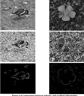
Figure 4.4 Comparison between polarity and gradient information ... 42

Figure 5.1 Comparison Results set no.1 ... 49

(11)

(12)

1 Introduction

1.1 Overview of computer vision

Computer vision, as a relatively new discipline, has the goal to enable

computers to “see”. The focused study of computer vision started in 1970

and it is still being investigated today. Computer vision is regarded as one

of the branches of artificial intelligence. Artificial intelligence intends to

simulate human behaviour in such a way that computer systems become

capable of performing functions that normally require human intelligence

e.g. reasoning, problem solving and learning from experience. Artificial

intelligence researches combine the elements of computer science and

cognitive psychology. Because of the difficulty of cognitive psychology

and human intelligence, most of the times computation stream is an

alternative which makes the machine to look intelligent. In computer

vision the aim is developing artificial vision systems that simulate human

vision.

Computer vision is a multidisciplinary research field and has been

overlapping with other fields such as computer graphics, image

processing, pattern recognition, and photogrammetry. These fields have

significant techniques and applications in common, while more briefly

computer graphics deals with creating images, image processing concerns

low level processing, pattern recognition extracts information from

signals mainly based on statistical approaches and photogrammetry is

obtaining highly accurate measurement using photographic images.

A growing number of applications exist for computer vision. One

prominent usage is in medical image analysis where data is in the form of

(13)

examples are detecting malign changes in samples or measuring the organ

dimensions. Military fields have been vastly improved by computer

vision advances. Missile guidance and autonomous vehicles are two

instances for this application. Also, computer vision is highly used in

industry for supporting a manufacturing process. An example could be

automatic quality control. Some of the other applications of computer

vision are robotic, surveillance and security, image data bases, virtual

reality, view synthesis and so on.

1.2 Definition of computer vision

Forsyth [Forsyth, 2003] described computer vision term as “Extracting

descriptions of the world from pictures or sequences of pictures”.

More detailed, computer vision can be defined as the study of

enabling the computers to acquire visual information, interpret this

information and act in response to this information. Computer vision

studies first deal with what kind of information is appropriate for the

system and should be captured from the input data i.e. from images.

Second, should find out how to extract this information. Next, come

across what is the most proper way to represent this information. At last

decide how to use this information in a system to perform its task

[Faugeras, 1993].

1.3 Motivations of the thesis

Segmentation is one of the sub domains of computer vision which has

been the subject of numerous researches. In object segmentation the main

purpose is to distinguish between the objects of interest and the rest of the

image. Most of the existing methods do this task while the object is

(14)

of techniques, as well as active contours assume that background has

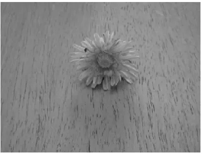
uniform intensity. Figure 1.1 shows an example of an object on a uniform

background.

Figure 1.1 object on a uniform background

Since the gradient in background of figure 1.1 is almost zero so the

contours are attracted to the edges of the flower without any problem.

One main problem in this field is the presence of noise and texture

outside the object. This means that, if the background is not clear enough,

the problem of object segmentation becomes more difficult. As we can

see in figure 1.2, the background has noise. The contour will be deviated

since it there are high gradient values in some regions other than the

objects borders.

(15)

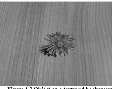
Figure 1.3 shows an example on a textured background. Same

problem may occur here. The active contour stops in the textured area

before reaching the salient object.

Figure 1.3 Object on a textured background

This thesis proposes a new technique, based on active contours, that

can detect objects' boundaries even when the background has noise

and/or texture. The proposed active contour model is aimed at providing

robust segmentation results for complicated cases with non-uniform

backgrounds. They are also applicable to any image segmentation

problem with clear and uniform background.

1.4 Overview of the thesis

The structure of the thesis is as follows: first image segmentation in

literature is studied. Different types of segmentation methods are

categorized in four groups: thresholding techniques, edge-based

techniques, region-based techniques and hybrid ones. In each group main

contributions are introduced and explained. The Third chapter discusses

active contours which are curves that deform and

move toward the objects' boundaries. In the context of active contours,

snakes and level set methods are studied. Chapter four represents our new

(16)

contains the experiments that show the robustness of the thesis proposed

(17)

2 Image segmentation

Objects need to be separated from the rest of the image. This is the first

step in image analysis which is the task of “image segmentation”. Image

segmentation is a long standing problem in computer vision.

Segmentation means organizing image content into semantically related

groups which are connected and homogenous. Some of the practical

applications of image segmentation are:

• Medical Imaging

o Locate tumors and other pathologies

o Measure tissue volumes

o Computer-guided surgery

o Diagnosis

o Treatment planning

o Study of anatomical structure

• Locate objects in satellite images (roads, forests, etc.)

• Face recognition

• Fingerprint recognition

• Traffic control systems

• Brake light detection

The result of image segmentation- the description of these objects-

will be used later in object representation and in feature measurement

process.

In this chapter after a brief description of image segmentation and

investigating “good” segmentation, classification of image segmentation

is studied. This classification is grouped in four main categories:

(18)

2.1 Definition

Formal definition for segmentation is [Horowitz, 1976]:

Segmentation of a grid X into X1,X2,...Xn subsets must satisfy the

following conditions, where P(Ri) is a uniformity predicate for all

elements in set R:

• Un_i₌1 X_i = X

• For i and j, if i≠ j, X_i ∩X_j =Ø

• P(X_i) = TRUE for all i

• P(Xi ∪Xj)= FALSE if i≠ j

The first condition implies that the collection of all the segments will

make the whole image. The second condition shows that two different

segments should not overlap. The third condition points out that the

pixels in one segment have the same properties all over the segment, and

the last condition presents that two different segments have dissimilar

properties.

Segmentation methods may use this definition or a variation of this.

However, there are cases that all these definitions are not enforced in the

algorithms.

2.2 What is a good segmentation?

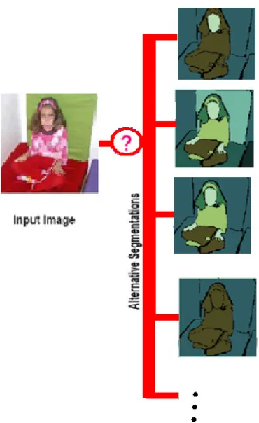
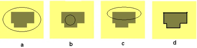
There are exponentially many possibilities to partition an image (figure

2.1). There is no single answer to the question: “What is a good

segmentation?”. It depends on what application we want to use

(19)

Figure 2.1 Different ways to segment an image

2.3 Classification of algorithms

By introducing the first edge detector, the image was officially

decomposed into its components. This could be considered as the first

image segmentation technique. The first edge detector, Roberts [Roberts,

1963], worked based on applying a 2×2 filter in sequence. The input for

this operator was a gray scale image and in the output each pixel was

showing estimated magnitude of the gradient. Although this detector is

fast but it is very sensitive to noise. A great number of methods have

emerged in segmentation since 1963, and still this topic is considered as a

challenging research topic.

There are many developed algorithms and there is more than one

classification of these algorithms. Image segmentation methods can be

(20)

use the traditional classification which classifies the image segmentation

methods into four categories: thresholding methods, edge-based

methods, region-based methods and hybrid methods that integrate-edge

and region-based ones.

2.3.1Thresholding

Among all the techniques in image segmentation, thresholding is

conceptually the simplest approach that we can take to separate the

objects from the background. Thresholding convert an image into a

binary image based on a threshold value ‘T’. Pixels are going to be

marked as object pixels if their intensity is greater than ‘T’. Otherwise, if

their intensity is less than ‘T’, they will be set as background.

Thresholding works well when objects and background have dissimilar

intensity distributions.

The goal in thresholding algorithms is to find an ideal threshold value

for getting the best segmented image. Thresholds can be adjusted either

manually or automatically. In manual threshold selection, a person should

give comments whether the threshold value is correct enough or not. This

process is time-consuming and objective. Errors may happen in selection

of ‘T’ and later more problems are produced in image analysis. For this

reason, a great number of methods have been introduced to automate the

thresholding process like [Melgani, 2006] [Sezgin, 2004] [Sauvola,

2000]. We are going to review some of the automatic methods in

followings.

One of the simplest thresholding methods is to find peaks and valleys

in histogram and set the threshold according to them. This approach is

robust because peaks can be easily found since their shape is well

(21)

and maximum are detectable. To avoid false peaks and valleys, the

histogram usually is smoothed. One algorithm based on peaks detection is

[Sezan, 1985] which at first finds zero-crossings and later uses a peak

detection signal to estimate significant peaks. One advantage of this

method is that we can adjust how fine the peaks are going to be. In

[Boukharouba, 1985] a variation of this method is used where the

cumulative distribution function of the image is first extended; pursued

by the curvature examination. More related methods can be found in

[Tsai, 1995] [Carlotto, 1987] [Olivo, 1994].

Rosenfeld [Rosenfeld, 1983] finds the optimal threshold through an

analysis of the convex deficiency which is calculating from deducting the

histogram from its convex hull. Some other modifications of this idea are

[Whatmough, 1991] [Sahasrabudhe, 1992].

One famous thresholding algorithm is Otsu’s [Otsu, 1979] method. In

this automatic unsupervised thresholding algorithm, distribution of pixels

value is analyzed. The basic idea here is that the pixels in each class

(cluster) should be as similar as possible. This means that the variance

inside each class should be minimized. Otsu defined the within-class

variance as the weighted sum of the variances of each cluster. Because

calculating within-class variance is expensive, we can use between-class

variance in computation instead. Minimizing within-class variance is

equivalent with maximizing between-class variance. Otsu’s method is

most widely employed in literature and its result is robust and

satisfactory. Many papers use Otsu’s method with slight modifications.

Two-Stage Multi-threshold Otsu method is introduced in [Huang, 2009]

developed to overcome the inefficiency of original Otsu by reducing the

iterations so that, the computation time will be much more less. In [Wu,

(22)

feasible and faster also, resulted better segments in image. More

applications can be found in [Wang, 2007] [Ali, 2004] [Junwei, 2007].

The Iterative Self -Organizing Data Analysis Technique (ISODATA)

[Ridler, 1978] was developed by Ridler and Calvard. Like Otsu, they use

the means of foreground and background but here search for the optimum

is locally, unlike in Otsu which is global. The algorithm starts by an

initial threshold which is equal to the half of the maximum gray level.

Binary image is generated based on this threshold. The mean value then

is computed for the current background and foreground. The new

threshold is then replaced with the average of the calculated means. This

process is repeated until the threshold reaches convergence. This method

is quite popular and does not need initial training for segmentation

process. However, convergence in short period of time sometimes is

inaccessible. DYNO (Dynamic Optimal Cluster seeking) algorithm [Tou,

1979] is a modification of ISODATA, with the ability of split and merge.

In [Jiang, 2008], they employ ISODATA technique for building

extraction in remote sensing. In medical image processing [Ding, 2004]

Self-Organizing Data Analysis Technique Algorithm was applied to

detect tissue damage in MRI images.

Niblack [Niblack, 1986] introduced a local thresholding algorithm

which moves a window across the image and calculates the local mean

and local deviation for the canter of window each time. He achieved the

threshold value by developing a function of the mean and the standard

deviation of the neighbourhood. Trier and Jain [Trier, 1995] tested

Niblack’s method and proved that it has best results comparing to any

other local thresholding methods. In [Sauvola, 2000], a heuristic variation

of Niblcack’s formula is used in which the standard deviation is

(23)

window size. The size of the window should be set so that it saves the

local details and suppresses noises. In [Zhao, 2008] Niblack’s method is

used in video text processing.

Some algorithms for thresholding are based on information theoretic

approach which was introduced by [Pun, 1980]. The entropy-based

techniques have proven to be successful and convincingly robust [Kapur,

1985] [Chang, 1994] [Luthon, 2004]. These techniques rely on

maximising the total entropy of both the object and background regions

to discover the suitable threshold. Some of these methods also use the

pixels' spatial information. More examples are in [Chang, 2006] [Sezgin,

2004].

Although Gray level thresholding is the simple, easy to grasp and fast,

but threshold selection is not always straightforward. The major

drawback of threshold-based approaches is that they often fail to find the

best separation between true positive signals and false positive signals

(noise), e.g. if the threshold is kept too low, a lot of true positive signals

maybe are not detected. Another alternative way to segment the image is

edge-based segmentation.

2.3.2Edge-based segmentation

Edge-based segmentation approaches relies on the edges found in images.

These edges represent the location of the discontinuities in gray level,

colour, texture, etc. Edge-based methods are based on the information

previously achieved by the edges in the image.

A variety of edge detector operators, which usually are named after

their inventors, exist in literature. The most famous ones are Prewitt

[Prewitt, 1970], Sobel [Sobel, 1978], Laplacian [Pratt, 1991], Canny

(24)

always showing the objects boundaries, the images which are resulted

from edge detection could not be an appropriate segmentation result by

itself. Therefore, edge detection is regarded as a prepossessing step. The

goal is to connect the relevant edges in such a way that the object

boundaries are produced.

There exist many methods which use different approaches to locate

the objects borders. These methods also use different quantity of former

information. The more former information is available, the better the

segmentation results will be. Otherwise, if there is not enough

information about boundaries, methods should employ more local

information about the image.

Sometimes some small edges appear in images, because of noise or

illumination changes. One group of methods try to use threshold to

eliminate these edges. The original idea is from Kundu and Mitra

[Kundu, 1987]. Finding a global threshold that works all over the image

is not achievable. Edges are usually thick as well. For the solution,

non-maximum suppression and hysteresis thresholding can be used as it was

introduced by the Canny [Canny, 1983] edge detector. Non-maximum

process checks if each pixel is local maximum along gradient direction.

Then suppress the points which are not local maximum. Hysteresis

checks if that maximum value of gradient value is large enough. If the

gradient of a pixel is above the high threshold, it will be declared as edge

pixel. Otherwise, if the gradient of a pixel is less than the low threshold, it

would be non –edge pixel. Any value between these two ranges is going

to be edge pixel if it is connected to any edge pixel. These papers use the

same ideas in image segmentation [Liu, 2000] [Tefera, 2002].

Using thresholds in finding edges usually ends in noisy results, and

(25)

considers the edges properties’ in the context of both ends of edges. Local

edge strength is raised if there are adequate evidences that borders may

exist. Studying the context hear, means investing the local neighbourhood

of the edge. Weak edges, which are located between two strong edges,

are considered as a boundary. An isolated edge, even strong one, without

a supporting context will not be considered as border. Hanson et al.

[Hanson, 1978] introduced a conventional edge context assessment. Later

Prager [Prager, 1980] modified his algorithm. According to Prager’s

method, three groups of edge patterns exist, which cause the confidence

in an edge to be modified: patterns in which the confidence of edge

would be increased, decreased or remain unchanged. The initial

confidence of an edge will be set as the normalized gradient value. Then,

“edge type” would be recognized based on the confidence of edge

neighbours. At last, the confidence of the edge will be modified based on

previous confidence and its type. This process will be repeated until the

confidence value converges to either 0 or 1. This method is comparatively

simple and noise robust. However, it often slowly flows and after larger

numbers of iterations, giving worse results than expected. In [Sher, 1992]

another approach, which is using probabilistic distribution of edge

neighbourhood, is presented. More recent applications of edge relaxation

can be found in [Czuni, 2001] [Moro, 2008].

Another edge-based technique is called boundary tracing. This

technique is performable after the image is over segmented; means that

the background and the foreground are already separated. Tracing inner

and outer boundary is part of this algorithm. Inner region border is part of

the region but outer border is not. This definition indicates that two

adjacent regions do not have a common border. To overcome this

(26)

hybrid technique. Extended borders utilize inner borders for the upper

and left sides of the object and outer borders for the lower and right sides.

Extended borders specify a common border between adjacent regions. A

more advanced method for extended boundary tracing was developed in

[Liow, 1991].

One way to connect edge segments is to trace from pixel to pixel

through potential edge points. Decision for every edge pixel is based on

the neighbour pixel gradient value and gradient orientation. Local edge

linking methods usually start at some arbitrary edge point and then

observe the points in neighbourhood. Edge linking is regularly followed

by post processing. Farag [Farag, 1991] detected the contours in two

stages: edge enhancement followed by edge linking. In [Gao, 1999] for

object extraction a low-complexity edge-linking algorithm in colour

images is designed. For finding global edges Hough transform, [Hough,

1962], named after Paul Hough, is a good option that decides which

tokens belong to which objects. Here the input for Hough transform is a

set of ‘n’ edge points, which are found formerly by an edge detector, and

the output is all the lines which these edge points are placed on. Instead

of x-y plane, each line is represented in a-b plane which is the slope and

the intercept of lines. All points, that lie on a line ‘S’ in x-y plane, have

lines in parameter space that intersect at the ‘a1’, ‘slope’, and ‘b1’,

Intercept of the line S. Later Duda et al. [Duda 1972] showed a more

efficient method by using polar parameterization. Generalized Hough

transform introduced in [Merlin, 1975] to find arbitrary shapes with

known orientation and scale. Generalized Hough transform with arbitrary

orientation and scale developed in [Ballard, 1981]. Hough transform has

imperfections including lack of accuracy and misleading results when

(27)

1993] tries to find a solution to solve the mentioned problems. Mapping

form image space to parameter space is replaced with converging

mapping to improve time complexity and accuracy. Some Applications to

the randomized Hough transform are in [Behrens, 2003] [Ding, 2005]

[Jean, 2004] [Xu, 2007].

Although edge-based methods produce clean and well defined

boundaries between different regions, they are likely to produce gaps

between boundaries. The necessity of complicated post-processing is

considered as one of the problems in this area. Another approach in

segmentation is region-based segmentation that comes in follow.

2.3.3Region-based segmentation

When we segment the image by judging only on the gray value of pixels,

the pixels are grouped into objects and taking no account of connectivity

property. In other words, pixels are classified independently of the

context. In region-based segmentation, uniformity within a sub-region is

the main issue, unlike the edge-based segmentation that discontinuity is

the main concern. The uniformity may be based on different properties

e.g. intensity, colour and texture. Based on the chosen property, the

complexity, the form and the quantity of former information vary in

segmentation method. Comparing to edge-based methods, in

region-based methods more coherent regions are created. However, judgment

over region membership is harder than applying edge detectors.

A simple approach in region-based segmentation is region growing.

The central idea in region growing is to start from a single pixel and grow

into a coherent region. The starting pixel is called the seed pixel. A

similarity measure is used for comparing every other pixel to the seed.

(28)

Various definitions exist for describing the similarity measure for

instance using pixel’s intensity value or average intensity value. The

Comparing stage could also be done in several ways, sometimes the

seed is the only reference. This makes the region very sensitive to the

seed selection. If every new pixel is compared with its neighbours,

sensitivity to seed is removed. But region growing will become so slow

and results may be far away from the original pixel. Another comparing

candidate is region statistics i.e. region mean, variance, etc. One seeded

algorithm in [Adams, 1994] works as follow: checks to see if a pixel

touches only on region by checking all the neighbours having the same

label. If so, the similarity measure between the new pixel and the region

is computed. Otherwise, if the new pixel touches more than one region,

the similarity to all the regions is calculated and smallest one is selected.

After the similarity is retained for the pixel, the pixel is put in

sequentially sorted list (SSL). This list is ordered according to similarity

attribute. In this algorithm, pixels having not same labelled neighbours

are labelled as boundary pixels. 3D extension of this algorithm is

employed in [Justice, 1997]. An approach using seeded region growing

with effective pixel labelling technique and automatic seed selection

process is introduced in [Fan, 2005]. Latest applications of seeded

growing segmentation are in [Wu, 2008] and [Gomez, 2007]. In region

growing (merging) if the comparisons are based on fine details, it will be

computationally expensive. And also, final outputs depend on seed points

and search strategy.

One other viewpoint for region-based segmentation is region splitting.

Contrary to region growing, the method starts with the whole image as a

single region then, splits into sub regions based on homogeneity criteria.

(29)

results are not the same even if both use a same similarity criterion. An

early work using region splitting is in [Ohlander, 1978] where splitting of

inhomogeneous regions is used to divide recursively the entire image

until homogeneous regions are found. In [Shulman, 2004] recursive

region splitting is used for evaluation of a single scene by testing

statistical homogeneity criteria after each split. If homogeneity has got

better, the split is accepted otherwise the split is undone.

The main flaw in region splitting is that the sub regions may have

adjacent regions with similar properties. Solution for this problem

suggests using split and merge together [Horowitz, 1976]. It is achievable

to take advantage of these two methods by combination them. First the

entire image is supposed as one region if, it is not homogenous it splits to

sub regions. Each sub region is checked iteratively and is divided if, it is

not homogenous. At the end these adjacent regions with same properties

merge [Fukada, 1980] [Chen 1980]. Split-and-merge method is more

efficient than split or merge. An adaptive split-and-merge method and a

review of region homogeneity testing are in [Chen, 1991]. Diamand et al.

[Diamand, 2003] extended the algorithm to 3D case images. They used

topological maps for the representation of segmentation states and in split

and merge process. In [Zhan, 2006], for detecting text on colour images

split-and-merge segmentation is used after a pre-processing enhancement.

For locating a diagnostic tumour from ultrasound images, a

split-and-merge technique is employed [Kwak, 2003].

A drawback of algorithms in this group is that in general they create

distorted boundaries since the segmentation typically is carried out at

(30)

2.3.4Hybrid methods

Examining the segmentation results of both edge-based and region-based

techniques leads to the conclusion that either edge-based or region-based

segmentation fails to produce accurate segments. As mentioned in

[Salotti, 1992], both approaches usually suffer from lack of information

for segmentation. Because of the segmentation problems in complex

images, using only one of these techniques will not lead to satisfactory

results. Integrating both approaches looks like a good solution. Yet,

achieving this goal is not easy because region-based and edge-based

segmentation are based on different ideas.

Time of fusion is one main property of hybrid methods. Considering

that the hybrid algorithms are grouped into embedded integration and

post processing integration [Munoz, 2003]. As it is obvious from the

names, in embedded segmentation, an edge-based operator segments the

image first then, the output information is used in a region-based

segmentation or, a region-based operator segments the image first and

then, the results are used in edge-based segmentation. But, in post

processing method both edge-based method and region-based method are

processing the image independently. Afterwards, all the output

information is used in a posterior fusion step.

The most usual way in embedded segmentation is integrating of edge

information with region-based segmentation during the decision making

in region growing procedure. In [Bonnin, 1989], plus the homogeneity

criterion, the edge information is also considered during split and merge

process. When there is no edge pixel in the regions and adjacent regions

are homogenous, the region grows. Similarly, [Healey, 1992] employs the

absence of edge pixels as a homogeneity criterion in 3D scenes. Besides,

(31)

accuracy since false negative results from edge detection have serious

consequences on segmentation. In [Lewis, 2002], edge information is

used as a decisive factor for the split and merge during sonar images

processing.

One kind of post processing hybrid methods is over-segmentation.

This method is about finding all the possible segments by strict

region-based segmentation. At the same time, all the edges are found by

edge-based segmentation. The results of region-edge-based method are checked with

edges to find out whether they are real boundaries or not. If there is no

correspondence for each boundary, it will be removed. Examples of this

type of hybrid segmentation are in [Pavlidis, 1990] and [Gagalowicz,

1986]. Another strategy for getting over-segmented image is to start with

one boundary detection technique to over segment the image. Then the

boundaries are verified by analyzing the chromatic and textural attributes

on each side of the contour. If the attributes are different on sides then,

the boundary is valid. This approach is used in [Philipp, 1996] and

[Fjortoft, 1997]. A More current case of over-segmentation is in [Guo,

2005] where the gradient is used to find the correct boundary of the

over-segmented image to prevent from the merging dissimilar regions.

In addition, post processing segmentation is a way for finding the best

approach in image segmentation in the absence of ground truth data.

Defining an appropriate stopping condition or setting suitable thresholds

in region segmentation were some issues in traditional region-based

methods. These problems can be solved using the evaluation function

which measures the degree of the excellence of a region-based

segmentation in line with its consistency with the edge map. If the region

(32)

segmentation is selected as the best one. Examples are in [Revol-Muller,

2000] and in [Hojjatoleslami, 1998].

2.4 Summary

Image segmentation partitions the image into semantically related groups

which are homogenous and connected. There are exponentially many

possibilities to segment an image and there are a lot of options for getting

correct segmentation. Based on prior information we have and kind of the

application we want to use the results in, the approach may differ.

Generally segmentation methods can be categorized as thresholding,

edge-based segmentation, region-based segmentation and hybrid

segmentation which is the integration of the both edge and region

segmentation techniques. Thresholding is the simplest image

segmentation method. A constant called a threshold is employed to

segment objects and background. In Edge-based segmentation, edges that

found in an image are the basis for segmentation. On the other hand in

region- based segmentation the homogeneity of the region is the main

issue. By integrating edge and region information hybrid segmentation

gives better results. That is the reason why some people use hybrid

(33)

3 Active contours

Studying and using active contours have leaded to promising results in

context of segmentation. As the methods discussed in previous chapter

are not fully capable of segmenting objects boundaries, active contours

are introduced as a solution. This approach is based on using deformable

contours that move under the influence of forces and are used to track

boundaries and motions. The idea of using a deformable pattern for

selecting particular features in image are introduced in [Widrow, 1973]

and in [Fischler, 1973] for the first time. However, it was not until the

work of [Kass, 1987] that the active contours became famous. The goal is

to find the equation that will drive the contour to the object. In other

words the curve should evolve until its boundary segments the object of

interest.

There are two deformable models: parametric models (snakes) and

geometric models (level sets). In parametric active contours, curves are

presented explicitly during deformation. On the other hand, in level sets

contours are shown as implicit level of functions which are based on

curve evolution and level set method.

In the following sections snakes are studied. Then a detailed review of

level set method is presented. Examples in literature for both techniques

are also introduced.

3.1 Snakes

The earliest and most famous active contour method is introduced by kass

[Kass, 1987]. Kass named his algorithm “snakes” because during the

evolution, the contours motion toward the object resembles snakes’

(34)

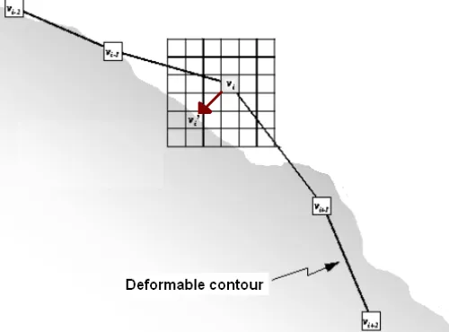
image, called initial contour, snakes locate the “actual” boundary. Let us

define a contour parameterized by arc length s as

C(s) = {( x(s), y(s)) : 0 ≤ s ≤ L}, R → Ω _(3.1)

Where L denotes the length of the contour C, and Ωdenotes the entire

domain of an image I(x, y). This algorithm is based on energy

minimization scheme. The basic idea of energy minimization is

minimizing the weighted sum of the internal energy, which depends on

the shape of the contour i.e. smoothness of the contour, and the external

energy which depends on image properties i.e. gradient.

ext

E E c

E( )= _int + _(3.2)

Minimizing the total energy yields internal forces and external forces.

Internal forces keep the curve together and prevent it from bending too

much. External forces draw the curve toward the desired object

boundaries. Each point is moved to the point, corresponding to the

place of the minimum value in (figure 3.1). If the energy functions are

chosen precisely, the contour, should move towards, and stop at, the

object boundary.

(35)

If αcontrols the tension of the contour and β controls the rigidity of the

contour, a common option for internal energy function will be:

ds s C s C E L 2 " 2 0 '

int =

∫

α ( ) +β ( )

(3.3)

The external energy function attracts the deformable contour to

interesting features, such as object boundaries, in an image.

∫

= E C c ds

E_ext _img( ( ))

(3.4)

A common option for edge attraction function is a function of image

gradient: R y x I G y x

Eimg Ω→

∇ = , ) , ( * 1 ) , ( σ λ (3.5)

Where Gσis a Gaussian smoothing filter and σ is its standard

deviation. Also λis a proper constant. To find the object boundary,

parametric curves are initialized within the image and are moved toward

the energy minima under the influence of both these forces. That is why

[He, 2008] refers to original snake as an interactive method which needs

expert guidance on the snake initialization and the choice of accurate

deformation parameters.

The classical snake limitations motivated other snake variations to be

introduced [Amini, 1990], [Cohen, 1991], [Zhu, 1996], [Xu, 1998],

[Giraldi, 2000], [McInerney, 2000], [Fenster, 2001], [Delingette, 2001],

and so on. Some of these limitations are as follows: since the magnitude

of the external force vanishes quickly as the contour diverges to the

boundaries and this makes the capture range of the snakes very small, the

(36)

contour is specified satisfactorily near the edges. Approximating a proper

location of initial contours without previous knowledge is usually a tricky

problem. In addition, snakes are very sensible to the noises in the image

can be easily distracted to wrong places. These were some drawbacks of

the original snakes but the most important flaw of classical snake is its

inability to adaptation of the model topology during the deformation. In

other words snakes maintain the same topology during the evolution

stage. That is, snakes cannot split to multiple boundaries or merge from

multiple initial contours.

In [Cohen, 1991] and [Xu, 1998] the focus is on reducing the

dependency on initial conditions by defining new external energy for

improving the snakes’ algorithm. Cohen et al. [Cohen, 1991] proposed a

new snake, called Balloon snake, and added a second external force

which shifts the contour out (inflation) or in (deflation) along its normal.

The new defined snake has resemblance to a balloon being inflated in 2D.

The balloon force enables the snake to be initialized inside the object in

addition to remove the necessity for the initial curve to be close to the real

edges. Comparing to the original snake by Kass [Kass, 1987], balloon

snake passes over relatively weak edges so has more stable results. Also,

if the object has a problematic shape, insertion a balloon inside the shape

and expanding its contour will locate the desired shape. However, balloon

snake has the problem with forcing the snake into concavities. Xu and

Prince [Xu, 1998] introduced gradient vector flow(GVF) snake which

increases the capture range and improve the snakes ability to move into

boundary concavities. It still has difficulties, however, forcing a snake

into lengthy, thin boundary indentations. Like the Cohen’s [Cohen,

(37)

vicinity. GVFs are vector fields derived from images by minimizing an

energy functional in a variational framework.

Both [McInerney, 2000] and [Delingette, 2001] try to help the

topology change during the evolution. In [McInerney, 2000]

topology-adaptive snakes or T-snakes are introduced for medical image

segmentation based on an affine cell image decomposition (ACID)

framework. The ACID provides a method for contour re-parameterization

and that allows T-snakes to split or merge; in other words adapting to the

topology of object. Yet only specific motions- inflating or deflating- is

applicable. Also re-parameterization is making the method complex and

expensive particularly in 3D. New physical constraints are introduced in

[Delingette, 2001] to control the contour deformation. In addition to

ability of splitting, the contours are kept separated by removing

overlapped snake areas. So that handling the topological changes plus

restoring contour separations as a procedure reduces the likelihood that

contours converge toward the boundaries of other object, are Delingette’s

[Delingette, 2001] method properties.

In [Fenster, 2001] first the shape of the object is achieved then the

shape information is used as constraint. The Contour evolves considering

this constraint so that the contour will not be captured by fake edges.

Region based features are used in [Zhu, 1996]. In this method boundary

deformation and region merging are done iteratively. Region based

information to the accompaniment of edge based data overcome the noise

in the image. But the problem in splitting the contour in multiple contours

still exists. Amini el al. [Amini, 1990] and Giraldi et al. [Giraldi, 2000]

used a dynamic programming approach instead of Kass’s [Kass, 1987]

(38)

estimation of higher order derivatives are omitted here and the numerical

stability is improved.

3.2 Level set methods

Geometric deformable models provide an elegant solution to address the

primary limitations of parametric deformable models. These models are

based on curve evolution theory and the level set method.

Level set method was first introduced in [Dervieux, 1980] and then

devised by Osher and Sethian [Osher, 1988]. For capturing moving fronts

in a wide range of problems, level set method has shown to be a robust

numerical option. Some fields using level set techniques are image

processing, computer vision and graphics. As mentioned by Tsai [Tsai,

2003], an implicit data representation of a hypersurface, set of PDEs that

govern how the surface moves, and the corresponding numerical methods

for implementing this on computers are building components of classical

level set method.

3.2.1Level set concept

The main idea of the Level set method can be described as follows. In an

open region Ω, Γ is a closed interface evolving with the velocity υ. The

goal is to analyze and compute the motion of the interface. Osher and

Sethian’s idea is to define an implicit smooth (Lipschitz continuous)

function φ(x, t) which represents the interface as the set where:

φ(x, t) = 0 if x∈ Γ

φ(x, t) <0 if x∈ Γin

(39)

Where Γin shows the area inside the interface and Γout shows the area

outside (figure 3.2).

Figure3.2 The construction of level set function

The evolution could be described by convecting the φ with the

velocity field υ on the interface:

+v.∇ =0

∂ ∂

φ φ

t (3.7)

If the normal component of v is υ N = v.

φ φ ∇ ∇

, where

∑

= = ∇ n i xi 1 2 φ

φ , the

equation (2.1) can be written using normal velocity:

+ ∇ =0

∂ ∂ φ φ N v

t (3.8)

These equations are Hamilton-Jacobi equations so that with suitable

restrictions the theory of viscosiy solutions [Crandall, 1983] picks out

unique Lipschitz continuous solution.

A useful property of this approach is that the level set function

remains a valid function while the embedded curve can change its

(40)

parametric active contours, such as computational simplicity and the

ability to change curve topology. Unlike the snake can start far from the

boundary and will converge to boundary concavities.

3.2.2Level set dictionary and technology

Key terms and some key technological advances in level set methods are

[Osher, 2003]:

1. The interface boundary Γ (t) is defined by

{

x φ(x, t) = 0

}. The

region is bounded and its exterior is defined by

{

x φ(x, t) > 0

}.

2. The unit normal N to Γ (t) is

N=

3. The mean curvature κ of Γ (t) is defined by

κ = -∇. ( φ φ

∇ ∇

)

4. The Dirac delta function concentrated on an interface is

φ φ δ( )∇

where δ(φ)is a one-dimensional delta function. 5. The characteristic function χof a region Ω(t) is

χ= H(-φ)

where H is a one-dimensional Heaviside function and

H(x) ≡ 1 if x>0

(41)

6. The surface (or line) integral of a function f over Γ is

( )

dx x

f Φ ∇Φ

∫

Rn

) ( δ

and The volume (or area) integral of f over Ω is

( )

dx H x f

∫

Φ Rn ) (

7. In many cases, φwill develop steep or flat gradients which cause

problems in numerical approximations. For preventing φ from

becoming too flat or too steep near the interface as well as keeping

the zero location unchanged, the distance reinitialization [Sussman,

1994] procedure reshapes a general level set function φ(x, t) by d(x,

t) which is the value of the distance from x to Γ (t), positive outside,

and negative inside.

Let d(x, t) be signed distance of x to the closest point on Γ. The

quantity d(x, t) satisfies∇d =1, d is positive outside and negative

inside and also is the steady state solution to

φ_t +sgn(φ0)(∇φ −1)=0,φ(x,τ =0)=φ0(x) (3.9)

Here φ0 shows the level set function before the reinitialization. For

most applications, the reinitialization is only needed for a

neighbourhood around the zero level set, and the diameter of this

neighbourhood depends on the discretization of the partial derivatives

in the PDE. This implies that only a few time steps in τare needed.

8. The basic level set method concerns a function φ which is defined

all over space. Obviously this is wasteful unless one only cares about

(42)

φ only near the zero level set. We may solve (3.7) in a

neighbourhood of Γ of widthm∆x, where m is usually 5 or 6. Points

outside this neighbourhood need not be updated by this motion. Thus,

this local method works easily in the existence of topological changes

and for multiphase flow.

3.2.3Numerics

Eq. (3.8) is Hamilton-Jacobi equation when normal velocity is dependant

of x, t and∇φ, Numerical methods should be used on uniform Cartesian

grid because of existence of singularities in solutions. The key ideas

involve monotonicity, upwind differencing, essentially non-oscillatory

(ENO) schemes, and weighted essentially non-oscillatory (WENO)

schemes [Osher, 1991] [Osher, 1988] [Jiang, 2000].

3.2.4Level set in segmentation

As mentioned before, level set method has been widely used because it

lets the contour to fit in angles, corners and topological changes. A

special case of the motion of the contour is based on mean curvature and

v is calculated with curvature of the curve. A basic version of the speed

functions that combine curvature and constant deformation were

proposed in [Caselles, 1993] and [Malladi, 1995]. A famous active

contour model based on mean curvature is introduced in [Caselles, 1993]

using the flowing equations:

(3.10)

Where is a constant pushing the curve when curvature becomes

(43)

curve moves with the speed ). And is

an edge dependent function so that the contour stops at desired boundary

where g disappears. Another formula for finding the zero level sets are

proposed in [Malladi, 1993].

(3.11)

Again is a constant. M1 and M2 are minimum and maximum value

of the magnitude of the gradient . When the speed vanishes the

evolving contour will stop and this happens at the highest gradients. Later

Caselles [Caselles, 1997] proved that the minimization of the contour

energy is even to the minimization of the contour length weighted by an

edge detection function in the Riemannian space. He integrated the curve

evolution methods with the classical energy minimization methods

(snakes). Other speed functions for evolving curves can be found in

[Siddiqi, 1998]. Often in level set methods the initial level set function is

frequently based on the signed distance. An efficient algorithm for

building of the signed distance function is called a fast marching method

[Malladi, 1996], [Malladi, 1998], [Sethian, 1999]. Applying the constant

deformation method may create sharp corners of the zero-level set

resultant in a vague normal direction. In that situation, the deformation

can be continued using an entropy condition [Sethian, 1982].

In classical geometric models, an evolution PDE for level set function

is originated from a certain evolution PDE of a parameterized curve. On

the other hand, in variational methods the evolution PDF of the level set

function is derived from minimizing the energy function defined on the

level set function. Comparing with classical methods, variational

(44)

In Zhao [Zhao, 1996] a variational level set method introduced.

Suppose there are disjoint regions Ωwith the boundaries Γso that the

common boundary between Ω_iand ΩjisΓ_i,_j. Energy function is described

as

2 1 E

E

E= + _(3.12)

Where E1 is the energy of the interface and E2 is the bulk energy. The

normal velocity is positive multiple of curvature of the interface plus the

bulk differences. That can be written as

dx H E dx E n

j j j n

i i i

∑

∫

∑

_∫

= = = ∇ = 1 2 1 1 ) ( ) ( φ γ φ φ δ γ (3.13)

Where H is Heaviside Function, δis delta function. Now minimizing

E is the sloution.

Chan et al. [Chan, 2001] came with new variational method without a

stopping edge-function, unlike the other level set methods that use

gradient value to stop the curve evolution. The original formulation of

Chan et al. [Chan, 2001] developed for bimodal images. This was

afterwards extended to multiphase images [Chan, 2002]. In the bi-modal

model, it is supposed that an image I is formed of two approximately

piecewise-constant distinct intensity regions, and . If the region to be

segmented is represented by , then a curve C can be evolved to reach

the boundary of by minimizing the energy:

(45)

(3.14)

,

(3.15)

The variables c1 and c2 show the average intensities inside, and

outside the curve respectively. It can be easily represent that the

minimum of the above fitting term is the boundary. If the curve is outside

the region then F2 and F1 > 0(figure 3.3 a), If the curve is inside

the region then F1 and F2 > 0 (figure 3.3 b), If the curve is both

inside and outside the region , then F2 and F1 > 0 (figure 3.3 c).

The only case that the fitting energy is minimized is when the curve is

located on the boundary (figure 3.3 d).

Figure 3.3 showing all the cases for the Chan & Vese method.

Chan and Vese [Chan, 2001] added some terms to the explained

function and introduced their energy function as:

(46)

Here ν µ are fixed parameters. By writing the area

and volume in energy form and

(3.17)

And

(3.18)

the function becomes:

(3.19)

By keeping the φ fixed and minimizing the F with respect to c1

andc2, the values of c1and c2 are calculated. Then they regularized δ and

H_{by two smooth functions}δε and Hε to use Euler-Lagrange equation:

0 ] ) ( ) ( . )[

( 2 0 2 2

2 1 0

1 − − − =

+ + ∇ ∇ ∇ − =

∂ F v λ u c λ u c

φ φ µ φ δε φ (3.20)

A way to solve this minimization problem is using gradient descent

on eq. (3.20) so that∂tφ =−∂φF .

The advantage of the Chan-Vese active Contours is that it is able to

segment an image even if it has smooth boundaries. The evolution of the

curve does not depend on gradient information; as a result weak edges do

(47)

initialization problems. The result of segmentation is dependent on the

situation of the initial curve.

The level set function φ can develop shocks which makes additional

computation vastly imprecise. A way to avoid this problem is to initialize

the function φ as a singed distance function, before the evolution and

then reshape the function φ to be a singed distance function periodically

during the evolution. In [Li, 2005] by mentioning to reinitialization’s

flaws such as the displacement of the zero level set within the

reinitialization, an increase of the number of iterations, nonexistence of a

known single method for reinitialization, making the computation more

expensive and complex; a new formula for geometric active contours

using new variational method has been discussed so that the is no need to

re-initialize the function. They define an energy function which consists

of internal and external energy. In order to keep the level set function as

an approximate signed distance function they use special internal energy

that penalizes the deviation of the level set function from a signed

distance function so that the level set function will be always close to sign

distance function. Sign distance function has the property =1 and any

function satisfying =1 is signed distance function. The internal

energy is

(3.21)

So that it shows how close a function is to its distance function. The final

energy function is

(48)

(3.23)

External energy function uses gradient function; it means that the

contour will be attracted to the points where the gradient is high:

(3.24)

(3.25)

Li’s method [Li, 2005] is computationally efficient, stable results are

produced and the most important advantage is omitting the reinitialization

process.

The use of level set and PDEs in computer vision has been developed

in recent years. In image segmentation many algorithms has utilized the

level set method to find “a collection of non-overlapping regions” of a

given image. There are a large variety of applications where which

geometric deformable models were employed for segmenting the image.

Examples include a level set-based cortical unfolding method

[Hermosillo, 1999]; cell segmentation [Sarti, 1996] and [Yang, 2005];

cardiac image analysis [Niessen, 1998], [Angelini, 2004], [Lin, 2003];

tumor tracking [Li, 2007], Biomolecular surfaces construction [Bajaj,

2008], and many others.

3.3 Summary

In this chapter, we have described the fundamental concepts of both

parametric and geometric deformable models and shown that they can be

Object Segmentation Using Active Contours: A Level Set Approach

Object Segmentation Using Active Contours: A Level Set

Object Segmentation Using Active Contours: A Level Set

Approach

Approach

By

Farnaz Shariat

A Thesis

Submitted to the Faculty of Graduate Studies

through the School of Computer Science

in Partial Fulfilment of the Requirements for

the Degree of Master of Science at the

University of Windsor

Object Segmentation Using Active

Contours:

A Level Set Approach

Windsor, Ontario, Canada

2009

Object Segmentation Using Active Contours: A Level Set

Approach

By:

Farnaz Shariat

Author’s Declaration of Originality

Abstract

Acknowledgements

Table of Contents

List of Figures

1

Introduction

1.1

Overview of computer vision

1.2

Definition of computer vision

1.3

Motivations of the thesis

1.4

Overview of the thesis

2

Image segmentation

2.1

Definition

2.2

What is a good segmentation?

2.3

Classification of algorithms

2.4

Summary

3

Active contours

3.1

Snakes

∫

∫

3.2

Level set methods

∑

{

}. The

{

}.

( )

∫

( )

∫

∑

∫

∑

∫

3.3

Summary

_∫