INVESTIGATION
Genome-Wide Patterns of Differentiation
Among House Mouse Subspecies
Megan Phifer-Rixey,*,1Matthew Bomhoff,†and Michael W. Nachman* *Museum of Vertebrate Zoology and Department of Integrative Biology, University of California, Berkeley, California 94720, and †BIO5 Institute, University of Arizona, Tucson, Arizona 85721
ABSTRACTOne approach to understanding the genetic basis of speciation is to scan the genomes of recently diverged taxa to identify
highly differentiated regions. The house mouse,Mus musculus, provides a useful system for the study of speciation. Three subspecies
(M. m. castaneus,M. m. domesticus, andM. m. musculus) diverged350 KYA, are distributed parapatrically, show varying degrees of
reproductive isolation in laboratory crosses, and hybridize in nature. We sequenced the testes transcriptomes of multiple wild-derived inbred lines from each subspecies to identify highly differentiated regions of the genome, to identify genes showing high expression divergence, and to compare patterns of differentiation among subspecies that have different demographic histories and exhibit different levels of reproductive isolation. Using a sliding-window approach, we found many genomic regions with high levels of sequence differentiation in each of the pairwise comparisons among subspecies. In all comparisons, the X chromosome was more
highly differentiated than the autosomes. Sequence differentiation and expression divergence were greater in theM. m. domesticus–
M. m. musculuscomparison than in either pairwise comparison withM. m. castaneus, which is consistent with laboratory crosses that
show the greatest reproductive isolation between M. m. domesticus andM. m. musculus. Coalescent simulations suggest that
differences in estimates of effective population size can account for many of the observed patterns. However, there was an excess of highly differentiated regions relative to simulated distributions under a wide range of demographic scenarios. Overlap of some highly differentiated regions with previous results from QTL mapping and hybrid zone studies points to promising candidate regions for reproductive isolation.
U
NDERSTANDING the genetic basis of speciation is afun-damental goal of evolutionary biology. This problem has primarily been approached in two ways: through laboratory studies using crosses and through studies of genetic variation in natural populations. Laboratory studies control for genetic background and environment, and they make it possible to connect genotype and phenotype. These types of studies have produced some spectacular successes including the identification of individual genes underlying postzygotic
iso-lation inDrosophila(e.g., Tinget al.1998; Presgraveset al.
2003; Brideau et al. 2006; Masly et al. 2006), Arabidopsis
(Bomblieset al.2007; Bikardet al.2009),Mus(Miholaet al.
2009), and others (reviewed in Presgraves 2010 and Nosil and Schluter 2011).
Studies of natural populations rely on the idea that regions of the genome that are important in reproductive isolation may be more differentiated than other regions of the genome. Therefore, by studying patterns of differentiation, one may gain insight into the genomic regions that underlie isolation. The idea that the genomes of closely related species are mosaics of differentiated and less differentiated regions is not
new andfirst emerged in the literature on hybrid zones (e.g.,
Key 1968; Harrison 1986; Tuckeret al.1992; Rieseberget al.
1999; reviewed in Harrison 2012). The advent of genomic methods has fueled a renewed interest in studying patterns of differentiation between closely related species, including
work on mosquitoes (Turner et al. 2005; Lawniczak et al.
2010; Neafsey et al. 2010), mice (Harr 2006), Drosophila
(Kulathinalet al.2009),Heliconiusbutterflies (Nadeauet al.
2012), flycatchers (Ellegren et al. 2012), crickets (Andrés
et al.2013), sunflowers (Renautet al.2013), and others.
Copyright © 2014 by the Genetics Society of America doi: 10.1534/genetics.114.166827
Manuscript received June 3, 2014; accepted for publication June 24, 2014; published Early Online July 3, 2014.
Supporting information is available online athttp://www.genetics.org/lookup/suppl/
doi:10.1534/genetics.114.166827/-/DC1.
1Corresponding author: The Museum of Vertebrate Zoology, University of California,
3101 Valley Life Sciences Bldg., Berkeley, CA 94720-3160. E-mail: [email protected]
Despite their appeal, genome scans present a number of challenges. One is correctly identifying genomic regions that show unexpectedly high levels of differentiation. This has typically been done either by specifying an appropriate null demographic model against which an observed distribution can be compared or by simply identifying extreme values as potential candidate regions. Another challenge is interpret-ing the biological meaninterpret-ing of a genomic region showinterpret-ing a high level of differentiation. Shared polymorphism can
result from retained ancestral variation or from gene flow;
conversely, differentiation can result from sorted ancestral variation (due to drift or selection) or from absence of gene flow. Charlesworth (1998) pointed out that reduced varia-tion within a populavaria-tion will inflate estimates of
differenti-ation, such as Fst, that are based on both within- and
between-population components of variation. As a result, background selection (Charlesworth 1993) and genetic hitchhiking (Maynard Smith and Haigh 1974) may lead to
localized high values of Fst even for regions that are not
involved in reproductive isolation (Cruickshank and Hahn
2014). Therefore, genomic “islands of differentiation”may
reflect (1) stochastic variation in lineage sorting; (2) regions
of reduced gene flow; (3) regions in which the effects of
selection at linked sites are more pronounced, regardless of involvement with reproductive isolation; or (4) some combination of these processes.
House mice provide a valuable system for the study of
speciation. Mus musculus consists of three subspecies that
are distributed parapatrically: M. m. domesticusin western
Europe, M. m. musculus in eastern Europe and northern
Asia, andM. m. castaneusin southeast Asia. These
subspe-cies are believed to have diverged in allopatry at roughly the
same time—350,000 years ago (Bonhomme et al.2007;
Geraldeset al. 2008, 2011; Whiteet al. 2009)—and come
into secondary contact much more recently (e.g., Cucchi et al. 2005; Duvaux et al. 2011). Each subspecies meets and hybridizes with the other two species where their
ranges come into contact (e.g., Tuckeret al.1992; Boursot
et al.1993; Duvaux et al.2011), although only the hybrid
zone betweenM. m. musculusandM. m. domesticusis
well-studied. Differences in estimated Ne among the subspecies
provide an opportunity to investigate the effects of demog-raphy on patterns of differentiation. While estimates of
ef-fective population size (Ne) are large for M. m. castaneus
(200,000–733,000), estimates are smaller forM. m.
domes-ticus(58,000–200,000) andM. m. musculus(25,000–120,000;
Salcedoet al.2007; Geraldeset al.2008, 2011; Halligan
et al.2010).
The degree of reproductive isolation differs in pairwise comparisons among house mouse subspecies. While
signif-icant reductions of F1male fertility are seen in crosses
be-tweenM. m. domesticusandM. m. musculus(e.g., Goodet al.
2008; White et al. 2011), significant infertility is not
ob-served until the F2in crosses between M. m. castaneusand
M. m. domesticus, and the degree of infertility is not as
se-vere (White et al. 2012). There are no published studies
documenting reduced fertility in lab crosses between M. m. castaneusandM. m. musculus. In fact, a cross between M. m. castaneus andM. m. musculuswas used for a recom-bination mapping study and infertility was not observed (Dumont and Payseur 2011).
In this study, we used short-read sequencing of the testis
transcriptomes of wild-derived inbred lines of M. m.
casta-neus,M. m. domesticus, andM. m. musculusto characterize genome-wide patterns of sequence differentiation in pair-wise comparisons between each subspecies. Although this study was primarily designed to investigate sequence differ-entiation, we also investigated patterns of differential gene expression among the subspecies.
Materials and Methods
Samples
All mice came from wild-derived inbred strains (Supporting
Information,Table S1). We sequenced eight lines ofM. m.
castaneus, seven of M. m. domesticus, and eight of M. m. musculus. Wild-derived laboratory strains of Mus spretus and Mus caroli were included for use as outgroups (She et al. 1990; Suzuki et al. 2004; Tuckeret al. 2005). Mice were killed and testes were dissected under RNAse-free con-ditions. Testes samples were kindly provided by François Bonhomme, Polly Campbell, Courtney Clayton, Matt Dean,
and Annie Orth. Testes were placed in RNAlater at 4°
over-night and then transferred to 280° for storage. RNA was
extracted from frozen tissue using Quiagen’s RNAeasy Plus
Mini Kit. Sequencing
Single-end 76-bp reads were sequenced from the mRNA of each individual on an Illumina GAIIx. For most lines, between 0.80 and 1.68 Gb of sequence was obtained (Table
S2). One wild-derived inbred line ofM. musculusand two
wild-derived lines selected from outgroup taxa were
se-quenced at higher coverage (1.92–3.64 Gb). Reads
contain-ing ,20 high-quality bases (phred $ 20) were removed
prior to mapping. Sequence data can be accessed via National Center for Biotechnology Information BioProject
PRJNA252743. TopHatv1.2 (Trapnellet al.2009) was used
with default settings to map reads to the C57BL/6 refer-ence genome, and only reads that mapped uniquely were
retained. Finally, sites with a depth ,63 of high-quality
sequence (phred $ 20) were removed from the analysis.
Thesefilters left between 12.01 and 22.70 Mb of sequence
per line. Genomic sequence data (.203) were available
from the Wellcome Trust Mouse Genomes Project for two of the lines included in our study (SPRET/EiJ and PWK/PhJ;
Yalcinet al.2012), and genomic sequence data were used to
augment transcriptome sequencing. We compared genotype calls between our data and the Wellcome Trust data in regions of overlap (Table S3). Although both data sets were obtained via shotgun sequencing, the higher coverage of the
Wellcome Trust data allows for an assessment of the possi-ble risks of sequencing and mapping using our lower-coverage approach. Mismatches were rare, occurring at rates ranging
from 1 in 325,000 to 1 in 420,000 coding sites (Table
S3). In addition, we included data from two lines (CAST/EiJ and WSB/Eij) sequenced only by the Wellcome Trust Mouse
Genomes Project (Yalcinet al.2012).
Previous analyses have shown that wild-derived inbred lines can contain large introgressed segments from other
subspecies (Yanget al.2011). STRUCTURE analysis (Pritchard
et al. 2000) was used to test for admixture in the wild-derived inbred lines sequenced in this study. We found that
two lines ofM. m. castaneusand one line ofM. m. musculus
were highly admixed, and we excluded them from the study (Table S1). After excluding these lines, the remaining sub-species formed three distinct groups corresponding to the three subspecies, and each line was assigned with most sup-port to the expected subspecies (Table S4). After removing the admixed lines and including the lines sequenced by the
Wellcome Trust, sixM. m. castaneus, eightM. m. domesticus,
and sevenM. m. musculuswere used in all analyses.
SAMtools was used with default settings to call bases and all SNPs within and among subspecies were identified using
custom PERL scripts (Liet al.2009;File S1). Inbred lines are
expected to be homozygous. Observed heterozygosity may reflect true residual heterozygosity in inbred lines or errors in sequencing; distinguishing between these two possibili-ties is difficult with low-coverage data. When heterozygosity was inferred using SAMtools, the site was masked and not included in further analyses. In addition, indels and sites with more than two segregating alleles were excluded. After filtering, we identified .32,000 SNPs within and among
subspecies ofM. m. musculusfrom 4705 genes with an
av-erage of 6.12 SNPs per gene. This represents 20% of the
genes in the genome.
Measures of sequence differentiation
There are many statistics for measuring differentiation, and these capture different aspects of the data. Here, we
cal-culated Fst(Hudsonet al.1992),Dxy(Nei 1987), and d,
the absolute value of the difference in allele frequencies (see
Renautet al.2010; Gagnaireet al.2012; equations given in
File S2) for each SNP for each pairwise comparison:M. m.
castaneus–M. m. domesticus(hereafter CD),M. m. castaneus– M. m. musculus(hereafter CM), andM. m. domesticus–M. m. musculus (hereafter DM). To account for unequal sample
sizes of the subspecies, we subsampled five lines per
sub-species 10,000 times at each site with sufficient data, and the average value of a given statistic was used for all sub-sequent analyses. Measures of differentiation were highly correlated in our data set (Table 1); thus we chose to use
d for subsequent analyses, although similar results were
obtained using other measures. We defined SNPs as highly
differentiated if average resampled values ofdper site were
$0.8. In such cases, the two subspecies are one allele or
fewer from fixation of alternate nucleotides. We defined
highly differentiated as d $ 0.8 rather than using an
ap-proach based on the distributions of statistics (e.g., the upper 5% of values) because it allowed us to compare among the three pairwise analyses. We then asked how many sites were fixed in a single subspecies but polymorphic in both of the
other two subspecies. Finally, we identified allfixed, derived
sites in each subspecies using comparisons to the outgroup
taxa,M. spretusandM. caroli.
Sliding windows
To identify genomic regions with groups of sites that are highly differentiated, we performed two kinds of
sliding-window analyses. First, sliding-sliding-window analyses of d
(100-kb windows with a 25-kb step size) were used to identify regions of the genome that were highly differentiated among subspecies. We defined regions as highly
differenti-ated if average values of d were $ 0.8 across all sites in
a window. All SNPs were included in these analyses, and windows were evaluated only when there were three or more SNPs in the window.
Private polymorphisms (i.e., those segregating in just one species) can lower the average level of differentiation in
a region as measured by Fst, Dxy, and d. The presence of
private polymorphisms does not mean that such regions are not potentially relevant to speciation, only that they are less likely, on average, to have experienced recent co-alescent events. Analyses that do not distinguish between shared and private polymorphisms may fail to identify many regions that are fully sorted. To address this problem, we
tracked the ratio of fixed differences to shared
polymor-phisms plus fixed differences using 100-kb windows with
a 25-kb step size. This ratio can take on values between zero and one and is defined for all regions that contain an in-formative site. High values indicate reciprocally monophy-letic gene genealogies while low values indicate populations that harbor ancestral polymorphism or are experiencing geneflow (e.g., Carneiroet al.2013). For this window anal-ysis, we included only windows with at least three topolog-ically informative SNPs.
In both sliding-window approaches, regions were de-limited by joining overlapping or adjacent windows with the same classification, and overall levels of diversity and differentiation were estimated by averaging across all SNPs in a delimited region. The average number of SNPs in these regions is given in Table 2. We also adopted a third ap-proach to defining regions of differentiation by delimiting
runs of fixed differences uninterrupted by shared
polymor-phisms. The results of these analyses were very similar to
the two sliding-window analyses and are given in File S2,
Figure S1,Table S5, andTable S6.
Demographic simulations
We used coalescent simulations (Hudson 2002) to compare observed patterns of differentiation to those expected under different demographic scenarios (Table S7). Parameters in these models included divergence time, current and ancestral
Ne, and migration rates in each direction and were based on maximum-likelihood estimates obtained using the program Isolation with Migration (IM) (Nielsen and Wakeley 2001)
in a previous study (Geraldes et al. 2011). We assumed no
recombination within loci and free recombination among loci. This assumption is reasonable given that linkage
disequi-librium decays over distances of 10–50 kb in house mice
(Laurieet al.2007). For each pairwise split, we simulated
100,000 gene genealogies, given five chromosomes from
each subspecies, and assumed a scaleduvalue of 1.33 based
on estimates of the mutation rate (4 3 1029; Waterston
et al.2002), ancestral population size, and the approximate average number of sites surveyed per locus. Because the program ms (Hudson 2002) simulates individual loci, we
then compared the distribution of d from the simulations
to the observed measures across individual genes in our data set. We also explored a wider range of demographic param-eters to better match simulated distributions to observed
values (seeResults).
Recombination and inversions
Regions of low recombination are expected to be more highly differentiated than other regions of the genome
(Noor et al. 2001; Rieseberg 2001; Nachman and Payseur
2012). For example, a recent study of sunflowers showed that regions of greater differentiation were strongly
associ-ated with reduced recombination (Renautet al.2013). We
used the revised genetic map to estimate the recombination
rate for 5-Mb intervals of the mouse genome (Shifmanet al.
2006; Cox et al. 2009). We defined low-recombination
regions as intervals with recombination rates falling in the bottom 10% of the genome and high-recombination regions as intervals falling in the top 10% of the genome. We then asked whether levels of differentiation differed between regions of low and high recombination. One limitation of
this approach is that the genetic map derives from M. m.
domesticus and there is some evidence that recombination rate varies among subspecies (Dumont and Payseur 2011;
Dumontet al.2011). This likely limits the power to detect
differences if they exist. To compare these results with
those from a previous study (Geraldeset al.2011), we
re-peated the analyses estimating recombination rates over 10-Mb intervals. We also repeated the analyses defining high- and low-recombination regions as those falling in the upper or lower 5, 15, and 20% of the distribution of re-combination rate.
Inversions may suppress recombination. Inversion data for M. m. castaneusand M. m. musculusrelative to the ref-erence mouse genome (C57BL/6) are available from the
Wellcome Trust (Yalcin et al. 2012). C57BL/6 is primarily
ofM. m. domesticusorigin but contains small introgressions from other subspecies. We used the Mouse Phylogeny
Viewer (Wang et al. 2012) to eliminate regions not of
M. m. domesticusorigin from the inversion data forM. m. cas-taneus and M. m. musculus. The location of inversions
be-tweenM. m. castaneusandM. m. musculuswas determined
Table 1 Sum ma ry statistics describing patte rns of di fferentia tion at all SNP s in pairw ise compa risons of the subspe cies of M. musc ulus Subsp ecies Sub species Chr omoso me No. of SNPs Fst (SD) Dxy (SD) d (SD)
rF;st Dxy
rF;dst rDxy
; d % fi xed di fferenc es % priva te poly morph isms % sh ared poly morph isms M. m. castan eus M. m. do mesticu s Auto somes 24,136 0.22 (0.3 2) 0.41 (0.28) 0.4 0 (0.29) 0.99 0.98 0.98 9.1 4 83.66 7.2 0 X 226 0.32 (0.4 1) 0.53 (0.34) 0.5 3 (0.35) 0.99 0.99 1.00 23.89 73.91 2.2 1 M. m. castan eus M. m. mu sculus Auto somes 23,709 0.26 (0.3 8) 0.44 (0.30) 0.4 3 (0.31) 0.97 0.98 0.99 12.50 81.55 5.9 5 X 237 0.35 (0.3 9) 0.54 (0.33) 0.5 3 (0.33) 0.97 0.98 0.99 18.14 73.00 8.8 6 M. m. domesti cus M. m. mu sculus Auto somes 21,598 0.38 (0.4 1) 0.53 (0.35) 0.5 2 (0.35) 0.98 0.99 0.99 24.01 70.96 5.0 3 X 246 0.46 (0.4 4) 0.57 (0.38) 0.5 7 (0.38) 0.99 0.99 1.00 30.08 68.29 1.6 3
by identifying and removing inversions in both lines that overlap and therefore represent inversions relative to M. m. domesticus. Many inversions were identified between
each pair of subspecies, but most were small (CD:x¼1762,
range = 99–19,005,n= 398; CM:x¼1907, range = 63–
19,752,n= 620; DM:x¼1749, range = 63–23,239,n= 479).
Therefore, variant SNPs in inversions were rare in our
data set. However, many runs offixed differences spanned
inversions. To investigate the relationship between
inver-sions and differentiation, we asked whether runs offixed
differences were more likely to overlap with inversions than expected by chance. To determine the expected overlap, we randomly generated the same number of regions across the genome sampled with replacement from the same size distribution as the runs data and de-termined the overlap with inversions. We did this 10,000 times and determined the percentile rank of the observed data.
Gene expression differences
The primary motivation for generating transcriptome data was to provide a set of common loci at which patterns of sequence differentiation could be analyzed. Nonetheless, these data also provide an opportunity to study gene expres-sion differences and to compare expresexpres-sion divergence with sequence differentiation.
All mice were unmated, reproductively mature males, but
they differed in age. In addition,M. m. domesticus
individu-als were reared in one facility while M. m. castaneus and
M. m. musculusindividuals were reared in another. We used two approaches to assess whether differences in rearing conditions might bias expression analysis. First, we cal-culated the average count of transcripts mapped for each gene in each subspecies correcting for differences in se-quencing effort. Pairwise comparisons between subspecies showed that expression patterns were highly correlated
(Pearson’s correlation; rCD. 0.99, d.f. = 15,123, P ,
10215; r
CM. 0.99, d.f. = 15,123, P, 10215; rDM. 0.99,
d.f. = 15,123,P,10215). Second, we compared our results
to those of another study on gene expression in M. m.
domesticus andM. m. musculus(M. Nachman, unpublished data). In that study, testis transcriptomes were sequenced
for three individuals of one inbred line ofM. m. domesticus
(LEWES) and three individuals of one inbred line ofM. m.
musculus (PWK). All mice were unmated, reproductively mature males of the same age, and all were housed in the same room of a single animal care facility. Average mean counts of transcripts mapped per gene for each subspecies after normalization were highly correlated in the two data
sets (rDOM Base Mean = 0.98, d.f. = 11,671, P , 10215;
rMUS Base Mean= 0.98, d.f. = 11,671,P,10215). In addition,
the log2fold change in expression for each gene between the
two subspecies was significantly correlated between the two
studies (rlog2 fold change= 0.71, d.f. = 11,671,P , 10215).
Although the power of the two studies differs due to design, the majority of genes (80%) identified in the smaller study
Table 2 Sum mary statistics des cribing regions identi fi ed as hi ghly di fferentia ted with a sliding-w indow ana lysis vs. all oth er regions in pairw ise comparis ons of the subspe cies of M. musc ulus Subsp ecies Subspec ies Chr omoso me Windo w type a n b Average size of region (bp ) c(SD) Aver age no. of SNPs (SD) Fst (SD) Dxy (SD) d (SD) p
d(SD)1
p
d(SD)2
M. m. castan eus M. m. dome sticus Autoso mes Hig hly differentia ted 63 133,33 3 * (37,56 7) 5.13 * (2.85) 0.80 * (0.1 0) 0.8 7 * (0.06) 0.87 * (0.0 6) 0.11 * (0.12) 0.05 * (0.07) Autoso mes All other s 1651 235,93 3 * (122,3 54) 13.74 * (13.67 ) 0.21 * (0.1 4) 0.4 0 * (0.12) 0.39 * (0.1 3) 0.26 * (0.11) 0.16 * (0.09) X Hig hly differentia ted 5 160,00 0 (33,54 1) 4.60 (2.30) 0.84 (0.1 5) 0.9 0 (0.09) 0.90 (0.0 9) 0.11 (0.15) 0.03 (0.04) X All other s 2 7 169,44 4 (37,55 3) 5.11 (2.87) 0.31 (0.2 3) 0.4 5 (0.20) 0.45 (0.2 0) 0.19 (0.17) 0.13 (0.11) All All 1746 230,98 5 (121,1 19) 13.27 (13.45 ) 0.24 (0.1 8) 0.4 2 (0.15) 0.41 (0.1 6) 0.25 (0.12) 0.15 (0.10) M. m. castan eus M. m. muscu lus Autoso mes Hig hly differentia ted 105 129,76 2 * (35,87 8) 5.31 * (2.84) 0.80 * (0.0 9) 0.8 7 * (0.06) 0.87 * (0.0 6) 0.11 * (0.10) 0.05 * (0.07) Autoso mes All other s 1625 229,70 8 * (114,9 47) 13.55 * (13.46 ) 0.24 * (0.1 5) 0.4 3 * (0.12) 0.41 * (0.1 3) 0.27 * (0.11) 0.14 * (0.11) X Hig hly differentia ted 6 154,16 7 (33,22 9) 3.67 (1.03) 0.86 (0.1 7) 0.9 2 (0.09) 0.92 (0.0 9) 0.03 (0.08) 0.12 (0.14) X All other s 2 6 168,26 9 (43,33 5) 5.38 (3.54) 0.32 (0.1 8) 0.4 9 (0.14) 0.48 (0.1 5) 0.21 (0.17) 0.16 (0.12) All All 1762 222,58 8 (113,6 26) 12.90 (13.14 ) 0.28 (0.2 0) 0.4 6 (0.16) 0.45 (0.1 7) 0.25 (0.11) 0.13 (0.11) M. m. domesti cus M. m. muscu lus Autoso mes Hig hly differentia ted 287 135,27 9 * (38,25 0) 5.98 * (3.62) 0.81 * (0.0 9) 0.8 7 * (0.06) 0.87 * (0.0 6) 0.07 * (0.07) 0.07 * (0.09) Autoso mes All other s 1561 216,94 4 * (111,4 86) 11.99 * (11.47 ) 0.34 * (0.1 7) 0.4 9 * (0.14) 0.48 * (0.1 4) 0.18 * (0.10) 0.15 * (0.11) X Hig hly differentia ted 4 162,50 0 (25,00 0) 4.75 (0.50) 0.90 (0.0 9) 0.9 3 (0.07) 0.93 (0.0 7) 0.04 (0.04) 0.05 (0.09) X All other s 3 3 170,45 5 (36,15 0) 4.97 (2.58) 0.38 (0.2 2) 0.5 0 (0.19) 0.50 (0.1 9) 0.11 (0.09) 0.15 (0.11) All All 1885 203,58 1 (106,8 56) 10.94 (10.79 ) 0.41 (0.2 3) 0.5 5 (0.19) 0.54 (0.1 9) 0.16 (0.10) 0.14 (0.11) * P , 10 2 10 in two-sided t-tests comparing h ighly differentiated autosomal regions and all other a utosomal regions in each pairwise comparison. aHighly differentiated regions de fi ned a s average d $ 0.8. bNumber o f d elimited regions. cRegions were d elimited by joining o verlapping or contiguous windows with the same classi fi cation. The resolution o f individual windows is limited to the sliding-window increment of 25,000. dp 1 and p2 refer to nucleotide d iversity (Nei and Li 1979) in the fi rst and second subspecies, respectively.
as having significantly different expression between the two
subspecies after correction for multiple testing (a = 0.01)
were identified as significantly differently expressed in this study after correction for multiple testing given a less
con-servative cutoff (a = 0.05). These analyses suggest that
expression patterns in this study were not strongly biased by differences in rearing conditions.
We identified genes that were differentially expressed in each pairwise comparison of subspecies. Given results from
TopHat (see above), HTseq (Anderset al.2014) was used to
create tables of counts of reads mapped for all represented
genes. All genes with an average read count of#10 in more
than one subspecies were removed from the analysis. The DESeq package in R (Anders and Huber 2010) was used to
further filter the data and identify genes with significant
differential expression using a binomial test. We first
nor-malized counts to account for differences in sequencing
ef-fort among individuals. We thenfiltered out the bottom 20%
of the data based on sums of the counts across all subspe-cies. This left 12,098 genes with sufficient data for analysis. We estimated dispersions for each subspecies and then used a binomial test to identify differentially expressed genes
be-tween each pair of subspecies. P-values were adjusted via
a Benjamini–Hochberg correction with a false discovery rate
of 0.01 (Benjamini and Hochberg 1995). Sites werefiltered
in each pairwise test if the average normalized read count
was#10 across both subspecies.
We estimated the correlation between measures of sequence differentiation on a gene-by-gene basis and the
absolute value of the log2fold change in expression for each
pair of subspecies. Sequence differentiation and expression differentiation might be correlated, particularly if differen-ces in expression are due to sequence changes at or near the
gene itself (i.e., cis-regulatory changes). In another study,
patterns of allele-specific expression in the testes of F1
hybrids ofM. m. domesticusandM. m. musculuswere used
to identify genes in which differences in expression between
the two subspecies were due to cis-regulatory changes (M.
Nachman, unpublished data) as in Wittkoppet al.2004. We
used those data and repeated the correlation analysis in the DM comparison, restricting it to genes identified as having cis-regulatory changes. Similar data were not available for the other two pairwise comparisons.
Testis-specific expression
Genes involved in reproduction are known to evolve quickly
(e.g., Begun et al. 2000; Wyckoff et al. 2000; Good and
Nachman 2005), and genes that are tissue-specific have higher rates of evolution than others in mammals (Duret and Mouchiroud 2000). We asked whether regions contain-ing testis-specific genes were more highly differentiated than other regions in the window analysis based on all SNPs. Genes with testis-specific expression were identified using
data from Su et al.(2004) available via BioGPS (Wuet al.
2009). Expression data were reduced to those tissues with support for independent expression, and expression values
were averaged over the available measurements for a given
tissue (Winter et al. 2004). Genes were considered
testis-specific if the proportion of total expression in the testis
compared to overall expression was $ 0.1 (Winter et al.
2004; File S3). Measures of differentiation for all regions
containing testis-specific genes were then compared to
mea-sures for all other regions using one-sidedt-tests.
Identifying candidate regions for reproductive isolation
One approach to identifying candidate genes for reproduc-tive incompatibilities is to look for overlap between the results of genomic scans and other methods such as QTL mapping studies and cline analyses in hybrid zones. There are many reasons to expect that the results of such studies will not overlap: QTL analyses focus on specific traits, hybrid zone data may track more recent processes, and genomic scans of differentiation will identify many regions that do not contribute to reproductive isolation. Nevertheless, inter-vals that are identified consistently across different methods are good candidates for additional study.
There are no published QTL mapping data of traits
relevant to reproductive isolation for crosses between M.
m. castaneusandM. m. musculus, nor are there any detailed hybrid zone studies between these taxa. However, there are published QTL mapping results for the other two pairwise
comparisons (Whiteet al.2011, 2012) and many studies of
the hybrid zone betweenM. m. domesticusandM. m.
mus-culus (e.g., Vanlerberghe et al. 1986, 1988; Tucker et al.
1992; Prageret al.1993; Munclingeret al.2002; Macholan
et al.2007; Teeteret al.2008, 2010; Janouˇseket al.2012). For QTL, we identified overlap between 1.5-LOD intervals associated with sterility phenotypes and highly differenti-ated regions in the window analysis based on all SNPs
(Whiteet al.2011, 2012). We combined QTL into a single
region for analysis if the QTL 1.5-LOD intervals were
over-lapping. For comparison with patterns in the musculus–
domesticus hybrid zone, we used the study by Janouˇsek et al. (2012) in which candidate Bateson–Dobzhansky– Muller incompatibility (BDMI) loci were identified from patterns of introgression and epistasis in two different transects. We identified overlap between a 2-MB window
centered on the candidate BDMI loci of Janouˇsek et al.
(2012) and highly differentiated regions in the window analysis based on all SNPs. For both types of comparisons, we compared the observed overlap to a distribution created using 10,000 simulated data sets of genomic regions from the same size distribution as those identified as highly dif-ferentiated in our study. We repeated all analyses identifying overlap between genes that were differentially expressed in our data and the results of previous studies. For these anal-yses, we compared the observed overlap to a distribution created using 10,000 simulated data sets. Simulations were conducted by sampling with replacement from among those genes for which there were expression data.
We used the coordinates of all SNPs in the Ensembl mouse genome assembly GRCm38 to identify genes found in
overlapping regions, and we used the Mouse Genome Database to identify phenotypes in laboratory lines
associ-ated with mutations in these genes (Eppig et al. 2012).
When highly differentiated regions wereflanked by regions
with fewer than three SNPs, we expanded the query regions to the next region with data or 2 MB, whichever was smaller. We did not include regions from the X chromosome as the QTL associated with male infertility in both crosses encom-passed most of the chromosome.
Results
Measures of sequence differentiation
Over 20,000 SNPs were segregating in each pairwise comparison, but many were private, segregating at low-to-moderate frequency within a single subspecies in a given
comparison (Table 1). Different measures of differentiation
(Fst,Dxy, andd) were highly correlated (Table 1). Average
levels of differentiation varied among pairwise comparisons, and all measures of differentiation were consistently higher in DM than in either of the other two pairwise comparisons. In addition, all measures of differentiation were higher on the X chromosome than on the autosomes (Table 1). Non-synonymous sites showed slightly lower levels of differenti-ation than synonymous sites in each pairwise comparison (Table S8).
There were 9529 individual SNPs that were highly
differentiated (d$0.80) in at least one of the three pairwise
comparisons (CD: 4223 from 1970 genes; CM: 5338 from 2343 genes; DM: 7423 from 2783 genes). Fewer SNPs were fixed inM. m. castaneusbut segregating in both of the other
lines (744 from 437 genes) than in eitherM. m. domesticus
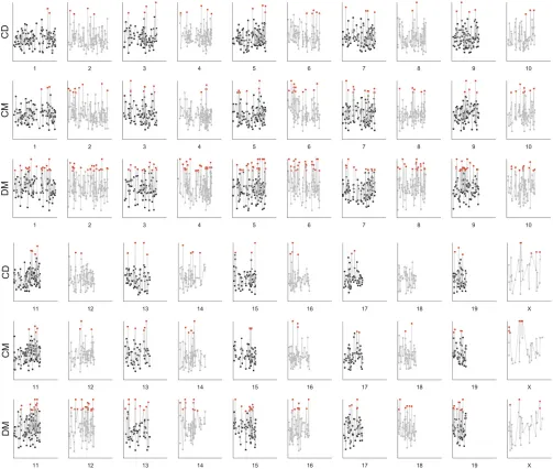
Figure 1 Sliding-window analysis showing average values ofdthroughout all chromosomes for each pairwise subspecies comparison (CD, M. m.
castaneus vs. M. m. domesticus; CM,M. m. castaneus vs. M. m. musculus; DM,M. m. domesticus vs. M. m. musculus). Each dot marks the start of
a delimited region, and red dots represent regions for which the average value ofdis$0.8.
(1084 from 651 genes) orM. m. musculus(1396 from 881 genes). In addition, many fewer sites represented derived states relative to the other subspecies and both outgroups in M. m. castaneus(372 from 263 genes) than in eitherM. m. domesticus (770 from 554 genes) orM. m. musculus(1570 from 1099 genes).
Sliding-window analyses
Thefirst sliding-window approach (based on average values
of d) included385–403 Mb in each pairwise comparison
afterfiltering (15% of the genome). We identified many
windows with an average value ofd$0.80 in each pairwise
comparison between subspecies (Figure 1 and Table 2). Highly differentiated regions were characterized by higher
measures of Fst and Dxy and lower measures of
within-subspecies variation than other regions (Table 2). Strikingly, regions of high differentiation represent a much larger part of the total surveyed transcriptome in the DM comparison than in either of the other two comparisons (Table 2). In
each pairwise comparison,.65% of genes sampled in highly
differentiated regions contained at least one fixed
differ-ence. Approximately half of those genes contained at least
one nonsynonymousfixed difference (CD: 57.4% of genes;
CM: 46.6% of genes; DM: 42.4% of genes). Although this implies that approximately half of these genes have no
non-synonymousfixed differences, it is important to bear in mind
that coverage was incomplete for many genes and thus some nonsynonymous changes may have been missed.
The second sliding-window approach (based on the ratio of fixed differences to shared polymorphisms plus fixed
differences), after filtering, included 89–146 Mb in each
pairwise comparison. This analysis required at least three topologically informative SNPs per window and thus
cov-ered much less of the genome than thefirst sliding-window
approach. We identified many fully sorted windows in each
pairwise comparison (Table 3;Figure S2, A–C). Even when
including private polymorphisms, autosomal regions that were fully sorted were characterized by higher measures
ofFst,Dxy,anddand by lower measures of within-subspecies
variation than other regions (Table 3). Notably, all regions on the X chromosome were fully sorted in all pairwise com-parisons. Fully sorted regions represent a much larger part of the total surveyed transcriptome in the DM comparison than in either of the other two comparisons (Table 3). As expected, a much higher proportion of the surveyed genome was identified as fully sorted in this analysis than was iden-tified as highly differentiated in the analysis averaging across all variable sites in a window.
Demographic simulations
We conducted coalescent simulations based on demographic
parameters estimated in a previous study (Geraldes et al.
2011; Table S7). The simulations predicted the greatest
overall levels of differentiation in the DM comparison and the lowest overall levels in the CD comparison (Figure 2),
a pattern consistent with the observed data. However, for all Tab
le 3 Sum ma ry statistics describin g patterns of differentia tion in fully sorted region s vs. all oth er region s in pairw ise comp arison s o f the sub species of M. muscu lus Sub species Su bspecies Chr omoso me type Window type a n b Aver age size of region (bp ) (SD) Aver age no. of SNPs (SD) Fst (SD) Dxy (SD) d (SD) p
c(SD)1
p
c(SD)2
M. m. castan eus M. m. dome sticus Autoso mes Fu lly sorted 223 15 9,193 (38,840 ) 15. 05 ** (9.17) 0.48 *** (0.1 6) 0.59 *** (0.1 3) 0.59 *** (0.13) 0.15 *** (0.1 0) 0.11 *** (0.07) Autoso mes All other s 321 15 7,243 (46,855 ) 19. 36 ** (12.56 ) 0.20 *** (0.1 3) 0.43 *** (0.1 0) 0.39 *** (0.11) 0.29 *** (0.0 9) 0.20 *** (0.09) X Fu lly sorted 5 1 7 5,000 (0) 5.20 (1.92) 0.80 (0.1 2) 0.85 (0.0 9) 0.8 5 (0.09) 0.06 (0.0 6) 0.0 5 (0.04) M. m. castan eus M. m. muscu lus Autoso mes Fu lly sorted 317 172,00 3 ** (52,573 ) 16.54 (10.86 ) 0.47 *** (0.1 7) 0.60 *** (0.1 3) 0.60 *** (0.13) 0.20 *** (0.1 0) 0.07 *** (0.06) Autoso mes All other s 287 154,35 5 ** (52,334 ) 18.20 (12.42 ) 0.19 *** (0.1 4) 0.42 *** (0.1 1) 0.38 *** (0.13) 0.28 *** (0.0 9) 0.21 *** (0.10) X Fu lly sorted 3 1 7 5,000 (0) 3.67 (1.15) 1.00 (0.0 0) 1.00 (0.0 0) 1.0 0 (0.00) 0.00 (0.0 0) 0.0 0 (0.00) M. m. dome sticus M. m. muscu lus Autoso mes Fu lly sorted 624 178,7 66 *** (55,386 ) 13.93 (9.50) 0.57 *** (0.1 7) 0.66 *** (0.1 3) 0.66 *** (0.13) 0.12 *** (0.0 7) 0.08 *** (0.06) Autoso mes All other s 234 140,17 1 *** (51,005 ) 14.50 (10.45 ) 0.27 *** (0.1 6) 0.48 *** (0.1 2) 0.44 *** (0.14) 0.22 *** (0.0 9) 0.23 *** (0.10) X Fu lly sorted 10 16,00 0 (24,152 ) 5.50 (1.27) 0.70 (0.1 8) 0.76 (0.1 5) 0.7 6 (0.15) 0.07 (0.0 6) 0.0 5 (0.06) * P , 0.05, ** P , 10 2 3, *** P , 10 2 7in two-sided t -tests comparing h ighly differentiated autosomal regions and all other autosomal regions in each pairwise comparison. aFully sorted regions are de fi ned a s those in which: # fixed differences # fixed differences þ # shared polymorphisms ¼ 1 (see Materials and M ethods ). bNumber o f d elimited regions. cp 1 and p2 refer to nucleotide d iversity (Nei and Li 1979) in the fi rst and second subspecies, respectively.
three pairwise comparisons, the observed distribution of d was flatter than the simulated distribution, resulting from a larger-than-predicted proportion of genes with extreme values. Differences between the observed and the simulated distributions were significant in all pairwise comparisons
(Kolmogorov–Smirnov test; CD: D2-sided = 0.23, P, 1 3
10210; CM:D
2-sided= 0.21,P,1310210; DM:D2-sided=
0.19,P,1310210). This pattern was most pronounced in
the CD and CM comparisons. An excess of genes with low values of differentiation is consistent with
higher-than-simulated rates of geneflow, whereas an excess of genes with
high levels of differentiation is consistent with longer-than-simulated divergence times, lineage-specific positive
selec-tion, and/or barriers to geneflow. However, on average, the
simulated loci had more variable sites than were surveyed in the observed data (Table S7). We repeated the simulations
choosing values of current and ancestralNeand divergence
time to try to match more closely the number of SNPs in the simulated and observed data (Table S9). Overall patterns were similar under both demographic scenarios (Figure S3
andFigure S4) with more loci falling in the extremes of the
distribution than expected based on the simulations. We further explored the simulation parameter space to
determine if increasing gene flow and divergence times
could generate patterns similar to those observed in the data. We started with the original parameter values (Table
S7) but with a common divergence time of 325 KYA. We
then explored different values of geneflow for each pairwise
comparison until the proportion of genes with low values of
differentiation (0,d#0.2) in the simulations matched the
proportion observed in the data. The levels of gene flow
required were high, ranging from 7 to 15 times the values originally simulated (Table S10). In all cases, increasing gene flow to the level required resulted in an even larger excess of highly differentiated genes in the observed data relative to the simulations than under the original demo-graphic scenario (Figure S4). Next, we tested whether
in-creasing divergence times in tandem with gene flow could
result in a distribution more similar to the one observed. We
increased the divergence timefirst to 425 KYA and then to
825 KYA. Increasing divergence time had little effect on the proportion of genes falling in the extreme tails of the
distri-bution for both the CD and CM comparison (Figure S5and
Figure S6). Increasing divergence times given such high
lev-els of gene flow tended to increase the proportion of
simu-lations for which the average value ofdwas low with little
effect on the proportion of highly differentiated loci. In the DM comparison, increasing divergence time did increase the proportion of the distribution that was highly differentiated
to levels close to or exceeding those observed (Figure S5and
Figure S6). However, in both simulations with older diver-gence times, the proportion of simulated loci with low val-ues of differentiation was much smaller than observed. We did not exhaustively explore the effects of uncertainty in estimates of effective population size, recombination rate, or mutation rate, any of which might affect the expected distribution of differentiation. Nonetheless, taken together, the simulations suggest that differences in demography can account for some of the observed patterns, such as increased differentiation in the DM comparison, but also that some regions of high differentiation result from either
lineage-specific positive selection or barriers to geneflow.
Recombination and inversions
Levels of differentiation were generally higher in regions of low recombination than in regions of high recombination, but the difference was significant only in the CM compar-ison. Results were similar among different measures of
differentiation; we report results ford(Table 4). Repeating
the analysis with 10-Mb windows or with different cutoff values for high- and low-recombination regions yielded qualitatively similar results (data not shown). We found no evidence of greater-than-expected overlap between
inversions and runs of fixed differences in the CM and
CD comparisons, but we did find significant overlap in
the DM comparison, with the observed overlap falling in
the extreme tail of the simulated distribution (P= 0.015;
Table S11)
Gene expression differences
We identified many more significantly differentially expressed genes in the DM comparison than in either of the other two
Figure 2 The distribution ofdvalues in the observed data and in the
simulated data based on demographic parameters from Geraldeset al. (2011).
comparisons (CD: 594 of 12,078; CM: 685 of 12,078; DM:
1049 of 12,081; File S4). Average d per gene and log2fold
change in expression were significantly positively correlated in all pairwise comparisons of subspecies, although the
corre-lation coefficients were small (CD:rd; absðlog2 fold changeÞ= 0.05,
d.f. = 2483,P= 0.01; CM:rd; absðlog2 fold changeÞ= 0.06, d.f. =
2471P= 0.001; DM:rd; absðlog2 fold changeÞ= 0.05, d.f. = 2356,
P = 0.02). Results were very similar for other measures of
differentiation (data not shown). Restricting the data to genes identified in another study as being significantly differentially
transcribed due to cis-regulatory changes (M. Nachman,
un-published data) strengthened the correlation in the DM com-parison although the significance was reduced given less
power (rd; absðlog2 fold changeÞ= 0.09, d.f. = 439,P= 0.05).
Testis-specific expression
Approximately 30% of regions surveyed in the analyses including all SNPs contained at least one testis-specific gene (Table S12). Overall, testis-specific genes were significantly more common in highly differentiated regions than in other
regions (x21 = 3.74, n= 9822, P1-tailed = 0.03). Regions
containing testis-specific genes were more differentiated than other regions in the CM and DM comparisons, but these differences were consistently significant only in the DM comparison (Table S12).
Identifying candidate regions for reproductive isolation between M. m. castaneus and M. m. domesticus
In comparisons between M. m. castaneusandM. m.
domes-ticus, we did not observe significant overlap between differ-entially expressed genes and QTL associated with hybrid male infertility. However, we did observe significant over-lap between highly differentiated regions and QTL (White et al. 2012; Figure 3A). Of the nine QTL intervals, seven contained peaks of high differentiation, and the observed overlap ranked in the 97th percentile of the simulated distribution.
Regions of overlap on the autosomes contained 221 protein-coding regions (Table S13). Across all 221 autoso-mal genes in regions of overlap, 20 genes were testis-specific
(BC049635,Bps9,Catsper2,Ccdc53, Ccl27a,Ccl27b,Eif3j1,
Faf1,Gm13306,Lin7a,Lrrc57,Nup37,Parpbp,Psmc3,Sord, Sycp3,Tex26,Trim69,Tsc22d4,Ttbk2), 11 genes had func-tional annotations and/or phenotypes associated with male
fertility (Arhgap1, Bps9, Cdkn2c, Celf1, Duox2, Ehd4, Igf1,
Illra1, Nr1h3, Pmch, and Pparg), and 3 genes were both testis-specific and had mutational variants associated with
male infertility (Catsper2,Sord,Sycp3). Nine genes in
re-gions of overlap showed significant expression differences
(padj ,0.05; 2700089E24Rik, Atg7, B2m, Capn3, Cdkn2c,
Igf1,Nup37,Ppip5k1,Shf). Two of those,Cdkn2candIgf1,
are associated with male fertility, and one,Nup37, is
testis-specific.
In general QTL are large, while regions of high differen-tiation are relatively small, potentially helping to narrow QTL intervals. For example, one QTL on chromosome 9 associated with amorphous sperm heads encompasses 26.7
Mb and contains 220 protein-coding genes (White et al.
2012). It overlaps with only one highly differentiated region
that contains only one protein-coding gene,Bbs9. Bbs9has
gene ontology (GO) terms relating to cilia and is testis-specific.
In humans, Bbs9mutations are associated with Bardet–
Biedl syndrome, a disease with multiple phenotypic effects
including reduced testis size. Expression levels atBbs9were
different in M. m. castaneusandM. m. domesticus, but this
difference was not significant after correction for multiple
testing (P,0.025,Padj = 0.16). We observed three silent
and no replacementfixed differences between M. m.
casta-neus andM. m. domesticus at Bbs9. Not all sites were sur-veyed, and thus observed patterns of differentiation may reflect linkage to functionally important unsurveyed sites. It is also important to bear in mind that not all genes in QTL intervals were surveyed.
Identifying candidate regions for reproductive isolation between M. m. domesticus and M. m. musculus
In comparisons betweenM. m. domesticusandM. m.
muscu-lus, the overlap between highly differentiated regions or dif-ferentially expressed genes and QTL associated with male
infertility (White et al. 2011) was not more than expected
by chance. The overlap between differentially expressed genes and candidate BDMIs loci from the hyrbid zone study
of Janouˇseket al.(2012) was also not more than expected by
chance. However, the overlap between highly differentiated regions and the candidate BDMI loci ranks in the 92nd
per-centile of simulated data (Janouˇseket al.2012). Regions of
overlap between all three kinds of studies (QTL, candidate BDMI loci from the hybrid zone, and regions of high differ-entiation) are particularly promising candidates for repro-ductive isolation. Importantly, six autosomal regions were identified in which candidate BDMIs and regions of high dif-ferentiation overlap precisely or are contiguous and fall within QTL intervals (Figure 3B). These regions collectively contain 242 genes, and the number of genes found in each specific region ranges from 17 to 97 (Table S14).
Two regions fall in relatively small QTL intervals. The first is on chromosome 4. This QTL is associated with
relative testis weight (Whiteet al.2011) and contains only
Table 4 Average sequence differentiation in regions of low and high recombination
Subspecies Subspecies dlow recombination(SD) dhigh recombination(SD) t P1-tailed n
M. m. castaneus M. m. domesticus 0.29 (0.12) 0.28 (0.06) 0.22 0.83 88
M. m. castaneus M. m. musculus 0.36 (0.10) 0.31 (0.05) 2.72 ,0.01 88
M. m. domesticus M. m. musculus 0.38 (0.13) 0.35 (0.07) 1.17 0.12 88
16 genes (Figure 4). Of these 16 genes, 4 are testis-specific
(4921539E11Rik, Mier1, Tctex1d1, and Wdr78) and two
(Insl5 and Dab1) are associated with male infertility. We
found that three genes (C8b,Dab1, andPrkaa2) in this
in-terval are differentially expressed betweenM. m. domesticus
and M. m. musculusafter correction for multiple testing
(a= 0.05).
The second small QTL interval with precise overlap is found on chromosome 5. This QTL is associated with both total abnormal sperm and distal bent-tail phenotypes. This interval contains 97 genes and is relatively well sampled in our study. There are 14 testis-specific genes in this interval
(Fbxo24,Mcm7,Mepce,Muc3,Myl10,Ppp1r35,Rabl5,Srrt,
Stag3, Taf6, Tmem184a, Tsc22d4, Znhit1, and Zscan21).
Two of these genes (Stag3 andZscan21) have GO
annota-tions and/or phenotypes relating to male fertility.Myl10and
Rabl5were differentially expressed betweenM. m. domesti-cusandM. m. musculusafter correction for multiple testing
(Padj,0.05). There are 10 additional genes in the region
with known functional annotations and/or phenotypes
re-lating to male fertility (Ache,Cnpy4,Cux1,Fam20c, Pdgfa,
Smok3a,Smok3b,Sun1,Vgf, andZan).
Discussion
Genome-wide patterns of sequence differentiation
We used a transcriptomic approach to characterize genome-wide patterns of differentiation between the three subspecies of house mice and discovered many highly differentiated regions in all pairwise comparisons. By comparing three
subspecies that split from one another at approximately the same time but that have different estimated effective population sizes, we were able to study the influence of demography on the early stages of speciation and di-vergence. In this case, we found higher levels of sequence
differentiation betweenM. m. domesticusandM. m. musculus
than between the other pairs of subspecies. This result is consistent with estimates of the demographic history of
these species; bothM. m. domesticusandM. m. musculus
are believed to have undergone significant bottlenecks
re-sulting in a currentNeof1/10 to 1/2 of the ancestralNe.
M. m. castaneus, on the other hand, is estimated to have a population size very similar to the ancestral population
(Geraldes et al. 2011). Lineage-specific changes observed
in this study support those expectations. The fewest
line-age-specific changes were assigned toM. m. castaneus, the
subspecies with the highestNe, and the most were assigned
toM. m. musculus, the subspecies with the smallestNe. More generally, the coalescent simulations performed here reca-pitulated the broad patterns of differentiation seen among the three subspecies, suggesting that many of the observed
patterns can be explained by differences inNeand levels of
geneflow (Figure 2).
At the same time, greater reproductive isolation is seen in
laboratory crosses between M. m. domesticusandM. m.
mus-culusthan betweenM. m. castaneusandM. m. domesticusorM. m. castaneusandM. m. musculus(Dumont and Payseur 2011;
White et al.2011, 2012). This observation, by itself, leads to
the prediction of greater differentiation in the DM comparison than in the other two comparisons. Because this pattern is also predicted by demographic differences among the subspecies, it is difficult to disentangle the relative contribution of differen-ces in demography and differendifferen-ces in reproductive isolation to the observed patterns. It is also unclear whether differences in demography are the cause of the differing levels of reproduc-tive isolation. For example, if most BDMI alleles were neutral on their own genetic background, then subspecies with smaller
Newould be expected to accumulate more BDMI differences
due to drift and would therefore show greater reproductive isolation. However, most BDMI genes in other systems seem to show evidence of positive selection, suggesting that drift is
not the predominant process fixing alleles involved in BDMIs
(Coyne and Orr 2004; Presgraves 2010). Differentiation on the X chromosome
The X chromosome was significantly more differentiated than the autosomes in all pairwise comparisons (Table 1). In principle, this pattern is expected for two reasons. First, the
smaller estimatedNeof the X chromosome should result in
faster lineage sorting. Second, this pattern is consistent with the large X effect, that is, the disproportionate accumulation of reproductive incompatibilities on the X chromosome (e.g., Coyne and Orr 1989). In this case, the greater level of dif-ferentiation appears to be more than can be explained by
differences in the X to autosome ratio ofNe. At
migration-drift equilibrium, assuming constant bidirectional migration,
Figure 3 Candidate regions for reproductive incompatibilities. (A)
Over-lap between autosomal regions identified as QTL associated with male sterility in a cross betweenM. m. castaneusandM. m. domesticus(blue bars) (Whiteet al.2012) and regions identified as highly differentiated in our scan based on all SNPs (black dots). (B) Overlap between QTL asso-ciated with male infertility (blue bars) (Whiteet al.2011), regions identi-fied as contributing to BDMIs betweenM. m. domesticus and M. m.
musculus in two-hybrid zones in central Europe (red dots) (Janouˇsek
et al.2012) and regions identified as highly differentiated in our scan
based all SNPs (black dots).
a sex ratio of 1, and equal migration of males and females,
Fst= 1/(4Nm+ 1) for the autosomes andFst= 1/(3Nm+
1) for the X chromosome. IfNmis0.1 (Table S7), then the
expected X:autosome ratio of Fst is 1.08 and the observed
ratios are 1.45 (CD), 1.35 (CM), and 1.21 (DM) (Table 1). This model is clearly overly simplistic. For example, there is some evidence of male-biased dispersal in this system
(Pococket al.2005). However, these rough calculations
sug-gest that differences in Ne alone cannot account for the
greater differentiation seen on the X chromosome.
On the other hand, our observations are consistent with previous work suggesting a large X effect. For example,
hybrid zone studies ofM. m. domesticusandM. m. musculus
indicate reduced introgression on the X (Tuckeret al.1992;
Dodet al.1993), and IM analysis of a limited number of loci
in all three subspecies suggests that gene flow on the
X chromosome is lower than that of autosomes (Geraldes et al.2008, 2011). In laboratory crosses, hybrid male steril-ity phenotypes map to the X chromosome in crosses between M. m. domesticusandM. m. musculus(Storchováet al.2004; Goodet al.2008; Whiteet al.2011) andM. m. castaneusand M. m. domesticus (White et al. 2012). Our findings here demonstrate that elevated differentiation on the X chromo-some is a general pattern, is observed in allopatric popula-tions, and extends to all pairs of subspecies.
Recombination
Several recent models suggest that chromosomal
rearrange-ments may lead to reduced gene flow via their effect on
suppressing recombination (Nooret al.2001; Rieseberg 2001;
Navarro and Barton 2003). Recombination can also influence differentiation by amplifying the effects of genetic hitchhiking and background selection within lineages (Maynard Smith and Haigh 1974; Charlesworth 1993), reducing variation within lineages and thus leading to increased differentiation between lineages. We found weak support for a negative relationship between differentiation and recombination, consistent with
these models. However, the power of this approach may be limited by the absence of data on recombination rate variation across the genome in all three subspecies.
Testis-specific expression
Regions of high differentiation contained a significantly higher proportion of testis-specific genes than other regions. This result is unexpected if highly differentiated regions simply reflect stochastic variation in lineage sorting. In contrast, this
result is consistent with (1) reduced geneflow due to BDMIs
associated with testis-specific genes, (2) hitchhiking effects associated with positive selection at testis-specific genes, (3) or both. Importantly, this observation suggests that some pro-portion of highly differentiated regions is associated with functional differences within or between nascent species. Candidate regions for reproductive incompatibilities
It would be incorrect to claim that all regions of high differentiation contribute to reproductive isolation when many such regions are expected simply as a consequence of drift in small populations. In addition, some regions of high differentiation are likely the result of lineage-specific se-lection that may not contribute to reproductive isolation. Nonetheless, the observed data differed from demographic simulations in one major way: the distribution of
differ-entiation statistics was flatter, with more values in the
extremes of the distribution. This is consistent with more gene flow and more differentiation than expected. Even
when exploring a broad range of values for geneflow and
divergence time, we were unable to find a demographic
scenario that recapitulated observed patterns. Therefore, some highly differentiated regions likely result either from lineage-specific positive selection and/or from barriers to geneflow at loci underlying incompatibilities.
One approach to prioritizing candidate reproductive iso-lation loci is to identify overlap between the results of genome scans, laboratory crosses, and hybrid zone analyses.
Figure 4 A region on chromosome 4 in which a QTL for relative testis weight (Whiteet al.2011), a candidate BDMI (Janousekˇ et al.2012), and a highly
differentiated region identified in this study overlap in the DM comparison. Testis-specific genes are given in italics, differentially expressed genes are underlined, and genes known to be related to male fertility are given in boldface type. All other genes are shown in grey.
We identified several areas of overlap between QTL
associ-ated with male sterility in a cross ofM. m. castaneusandM.
m. domesticus (Whiteet al.2012) and highly differentiated regions identified in our study. The overlap was more than expected by chance, but in most cases QTL were large, mak-ing the overlap difficult to interpret (e.g., chromosome 5, Figure 3A). However, in other cases, the QTL intervals were narrower, there was reasonable coverage in our data set, and relatively few genes were found in the overlap. For example, on chromosome 9, there is just one gene in a region of high differentiation that falls in a moderately sized QTL. Even
though .200 genes fall in all of the areas of overlap, this
number is considerably smaller than the total number of
genes that fall in QTL intervals (Whiteet al.2012). Moreover,
fewer than 3 dozen of those genes have known phenotypes or GO terms that relate to male fertility and/or are testis-specific as might be expected if they affect male sterility phenotypes measured in the QTL analyses. Of course, GO annotation and documentation of phenotypes associated with mutations or knockouts in mice are far from complete, and additional genes in these regions may be related to fertility.
In the DM comparison, overlap between our results and QTL analyses was considerable, but not more than expected by chance. More promisingly, there was meaningful overlap
between candidate BMDIs (Janouˇseket al. 2012) and our
results. In particular, there were six cases in which regions identified as highly differentiated in our study were directly overlapping or contiguous with a candidate BDMI and fell in a QTL interval. In two of those cases, the overlap was rela-tively precise, and the region of overlap contains a short list of genes that are testis-specific, differentially expressed, and/or related to male infertility. While there is still much work to be done, the intersection of results from multiple studies is encouraging and highlights the promise of this approach for narrowing QTL intervals.
Acknowledgments
We thank F. Bonhomme, P. Campbell, C. Clayton, M. Dean, and A. Orth for providing tissue samples; J. MacDonald for providing access to the source code for the program DNA Slider; and members of the Nachman Lab, D. Begun, D. Matute, and one anonymous reviewer for their thoughtful comments on the manuscript. This research was funded by National Institutes of Health grant R01 GM074245 to M.W.N. This work used the Extreme Science and Engineer-ing Discovery Environment, which is supported by National Science Foundation grant ACI-1053575.
Literature Cited
Anders, S., and W. Huber, 2010 Differential expression analysis
for sequence count data. Genome Biol. 11: R106.
Anders S., P. T. Pyl, and W. Huber, 2014 HTSeq: a Python
frame-work to frame-work with high-throughput sequencing data. bioRxiv DOI: 10.1101/002824.
Andrés, J. A., E. L. Larson, S. M. Bogdanowicz, and R. G. Harrison,
2013 Patterns of transcriptome divergence in the male
acces-sory gland of two closely related species offield crickets.
Genet-ics 193: 501–513.
Begun, D. J., P. Whitley, B. L. Todd, H. M. Waldrip-Dail, and A. G.
Clark, 2000 Molecular population genetics of male accessory
gland proteins in Drosophila. Genetics 156: 1879–1888.
Benjamini, Y., and Y. Hochberg, 1995 Controlling the false
dis-covery rate: a practical and powerful approach to multiple
test-ing. J. R. Stat. Soc., B 57: 289–300.
Bikard, D., D. Patel, C. L. Metté, V. Giorgi, C. Camilleri et al.,
2009 Divergent evolution of duplicate genes leads to genetic
incompatibilities withinA. thaliana. Science 323: 623–626.
Bomblies, K., J. Lempe, P. Epple, N. Warthmann, C. Lanz et al.,
2007 Autoimmune response as a mechanism for a
Dobzhansky-Muller-type incompatibility syndrome in plants. PLoS Biol. 5: e236.
Bonhomme, F., E. Rivals, A. Orth, G. R. Grant, A. J. Jeffreyset al.,
2007 Species-wide distribution of highly polymorphic
minisatel-lite markers suggests past and present genetic exchanges among house mouse subspecies. Genome Biol. 8: R80.
Boursot, P., J. C. Auffray, J. Britton-Davidian, and F. Bonhomme,
1993 The evolution of house mice. Annu. Rev. Ecol. Syst. 24:
119–152.
Brideau, N. J., H. A. Flores, J. Wang, S. Maheshwari, X. Wanget al.,
2006 Two Dobzhansky-Muller genes interact to cause hybrid
lethality in Drosophila. Science 314: 1292–1295.
Carneiro, M., S. J. E. Baird, S. Afonso, E. Ramirez, P. Tarrosoet al.,
2013 Steep clines within a highly permeable genome across
a hybrid zone between two subspecies of the European rabbit.
Mol. Ecol. 22: 2511–2525.
Charlesworth, B., 1993 The evolution of sex and recombination in
a varying environment. J. Hered. 84: 345–350.
Charlesworth, B., 1998 Measures of divergence between
popula-tions and the effect of forces that reduce variability. Mol. Biol.
Evol. 15: 538–543.
Cox, A., C. L. Ackert-Bicknell, B. L. Dumont, Y. Ding, J. T. Bellet al.,
2009 A new standard genetic map for the laboratory mouse.
Genetics 182: 1335–1344.
Coyne, J. A., and H. A. Orr, 1989 Patterns of speciation in
Dro-sophila. Evolution 43: 362–381.
Coyne, J. A., and H. A. Orr, 2004 Speciation. Sinauer Associates,
Sunderland, MA.
Cruickshank, T. C., and M. W. Hahn, 2014 Reanalysis suggests
that genomic islands of speciation are due to reduced diversity,
not reduced geneflow. Mol. Ecol. 23: 3133–3157.
Cucchi, T., J.-D. Vigne, and J.-C. Auffray, 2005 First occurrence of
the house mouse (Mus musculus domesticus SCHWARTZ &
SCHWARTZ, 1943) in Western Mediterranean: a revision of sub-fossil house mice occurrences using a zooarchaeological
critical grid. Biol. J. Linn. Soc. Lond. 84: 429–445.
Dod, B., L. S. Jermiin, P. Boursot, V. H. Chapman, J. T. Nielsen
et al., 1993 Counterselection on sex chromosomes in the
Mus musculusEuropean hybrid zone. J. Evol. Biol. 6: 529–546.
Dumont, B. L., and B. A. Payseur, 2011 Genetic analysis of
genome-scale recombination rate evolution in house mice. PLoS Genet. 7: e1002116.
Dumont, B. L., M. A. White, B. Steffy, T. Wiltshire, and B. A.
Payseur, 2011 Extensive recombination rate variation in the
house mouse species complex inferred from genetic linkage
maps. Genome Res. 21: 114–125.
Duret, L., and D. Mouchiroud, 2000 Determinants of substitution
rates in mammalian genes: expression pattern affects selection
intensity but not mutation rate. Mol. Biol. Evol. 17: 68–070.
Duvaux, L., K. Belkhir, M. Boulesteix, and P. Boursot,
2011 Isolation and geneflow: inferring the speciation history
of European house mice. Mol. Ecol. 20: 5248–5264.