Wojtys, M and Marra, G. and Radice, Rosalba (2016) Copula regression
spline sample selection models: the R Package SemiParSampleSel. Journal
of Statistical Software 71 (6), ISSN 1548-7660.
Downloaded from:
Usage Guidelines:
Please refer to usage guidelines at or alternatively
MMMMMM YYYY, Volume VV, Issue II. http://www.jstatsoft.org/
Copula Regression Spline Sample Selection Models:
The
R
Package
SemiParSampleSel
Ma lgorzata Wojty´s University of Plymouth Warsaw University of Technology
Giampiero Marra University College London
Rosalba Radice Birkbeck University of London
Abstract
Sample selection models deal with the situation in which an outcome of interest is observed for a restricted non-randomly selected sample of the population. The estimation of these models is based on a binary equation, which describes the selection process, and an outcome equation, which is used to examine the substantive question of interest. Classic sample selection models assume a priori that continuous covariates have a linear or pre-specified non-linear relationship to the outcome, and that the distribution linking the two equations is bivariate normal.
We introduce the Rpackage SemiParSampleSel which implements copula regression
spline sample selection models. The proposed implementation can deal with non-random sample selection, non-linear covariate-response relationships, and non-normal bivariate distributions between the model equations. We provide details of the model and algorithm and describe the implementation inSemiParSampleSel. The package is illustrated using simulated and real data examples.
Keywords: copula, non-random sample selection, penalized regression spline, selection bias,
R.
1. Introduction
The sample selection model was introduced by Gronau (1974), Lewis (1974) and Heckman
(1976) to deal with the situation in which the observations available for statistical analysis are not from a random sample of the population; the model was discussed byHeckman(1990)
among others. This issue occurs when individuals have selected themselves into (or out of)
con-ducted in the United States between 1974 and 1982 (Newhouse 1999) which will also be ana-lyzed in Section5. The aim was to quantify the relationship between several socio-economic characteristics and annual health expenditures. Non-random selection arises if the sample consisting of individuals who used health care services differ in important characteristics from the sample of individuals who did not use them. If the link between the decision to use the services and health expenditure is through observables, then selection bias can be avoided by accounting for these variables. However, if the link is through unobservables as well then inconsistent parameter estimates are obtained when using a classic univariate equation method. There are two more aspects that may complicate modeling the relationship between covariates and annual health expenditure. Variables such as age and education are likely to have a non-linear relationship to both decision to use health services and amount to spend on them; this is because they embody productivity and life-cycle effects that are likely to have non-linear effects. Imposing a priori a linear relationship (or non-linear by simply using quadratic polynomials, for example) could mean failing to capture the true more complex
relationships. Finally, the (often criticized) assumption of bivariate normality (employed in
many sample selection models) between decision to use health services and expenditure may be too restrictive for applied work and is typically made for mathematical convenience.
The literature on sample selection models is vast and many variants of such models have been proposed. Chib, Greenberg, and Jeliazkov (2009) and Wiesenfarth and Kneib (2010) introduced two estimation methods to deal with non-linear covariate effects. Specifically, the approach of the former authors is based on Markov chain Monte Carlo simulation techniques and uses a simultaneous equation system that incorporates Bayesian versions of penalized smoothing splines. The latter further extended this approach by introducing a Bayesian al-gorithm based on low rank penalized B-splines for non-linear and varying-coefficient effects and Markov random-field priors for spatial effects. Recently,Marra and Radice (2013) pro-posed a frequentist counterpart which has the advantage of being computationally fast and can especially appeal to practitioners already familiar with traditional frequentist techniques.
Under the assumption of bivariate normality Heckman (1979) proposed a two-step
estima-tor. However because the estimator is inconsistent under distributional misspecification
var-ious methods that relax the assumption of normality have been proposed over the years; these include semiparametric(e.g.,Gallant and Nychka 1987;Powell, Stock, and Stoker 1989;
Ahn and Powell 1993;Lee 1994a,b;Powell 1994;Andrews and Schafgans 1998; Newey 2009)
and nonparametric methods (e.g., Das, Newey, and Vella 2003; Lee 2008; Chen and Zhou
2010). Another way to relax the normality assumption is to use non-normal parametric distributions. Recently,Marchenko and Genton(2012) andDing(2014) extended the sample selection model to deal with heavy tailedness by using the bivariate Student-t distribution. Another parametric method, which includes as a subcase the above mentioned Student-t approach, is copula modeling. This allows for a great deal of flexibility in specifying the joint distribution of the selection and outcome equations (e.g., Smith 2003; Prieger 2002;
Hasebe and Vijverberg 2012;Schwiebert 2013).
In summary, the numerous estimation approaches that deal with the assumption of normality in the sample selection model can be divided into two large groups: semi/non-parametric and flexible parametric estimators. The first relaxes the assumption of bivariate normality by us-ing a general bivariate density function, whereas the second offers the possibility of replacus-ing bivariate normality with an alternative parametric stochastic structure. There are advantages
strongest point of the semi/non-parametric approach is the property of maintaining consis-tency of such estimators even disposing, in part or altogether, of distributional assumptions. In some cases, simplified versions of these methods are easy to implement (e.g., Das et al.
2003). However, these estimators do have shortcomings. Specifically, semi/non-parametric methods are usually restricted when it comes to including a large set of covariates in the model and the resulting estimates are inefficient relatively to fully parametrized models (e.g.,
Bhat and Eluru 2009). To date, packages implementing semi/non-parametric procedures are CPU-intensive and the set of options provided is often quite limited. In addition, convergence problems are likely to occur when using models which include, for instance, many discrete vari-ables and interactions. As for the parametric approach, many scholars agree upon its greater computational feasibility as compared to semi/non-parametric approaches, which allows for the use of familiar tools such as maximum likelihood without requiring simulation methods or numerical integration. As pointed out by Smith (2003), maximum likelihood techniques allow for the simultaneous estimation of all model parameters, and such methods, if the usual regularity conditions hold and the model is correctly specified, ensure consistent, efficient and asymptotically normal estimators. In addition, when using copulas the practitioner has the possibility of a piece-wise model specification. This is because marginal distributions are not constrained to belong to the same family of the chosen bivariate copula distribution. More-over, Genius and Strazzera (2008) argue that copula modeling allows for direct estimation of the dependence structure in the sample selection model while non-parametric methods do
not. However, a crucial point stands on the correct specification of these models; maximum
likelihood estimators are not consistent when the distributional assumption is not correct.
Also, testing the distributional assumption is not straightforward. In the context of
Heck-man’s two-step estimator,Lee(1982,1984) presented misspecification tests based on bivariate
Edgeworth expansions. Recently, Montes-Rojas (2011) proposed a similar methodology for
testing normality in sample selection models. Specifically, he proposed Lagrange multiplier
and Neyman’sC(α) tests for the marginal normality and linearity of the conditional
expecta-tion of the error terms for the two-step estimator. Although these tests provided encouraging results, more research is necessary to construct likelihood ratio and Wald tests. As for the maximum likelihood approach, to date, all that can be done is a posteriori model selection
using, for instance, traditional information criteria.
Some of the methods described above are implemented in popular software packages likeSAS
(SAS Institute Inc. 2011), Stata(StataCorp 2011) and R(RDevelopment Core Team 2013).
For example, the conventional Heckman sample selection model can be fitted in SAS
us-ing the proc qlim and in Stata using heckman. The non-parametric method by Lee (2008)
can be employed using the Stata package leebounds and the bivariate Student-t
distribu-tion Heckman model using heckt. In R the sample selection packages are sampleSelection
(Toomet and Henningsen 2008), bayesSampleSelection(Wiesenfarth and Kneib 2010), avail-able from the first author’s webpage, ssmrob (Zhelonkin, Genton, and Ronchetti 2013) and
SemiParBIVProbit (Marra and Radice 2014). sampleSelection and bayesSampleSelection
make the assumption of bivariate normality between the model equations. sampleSelection
andssmrobassume a priori that continuous regressors have linear or pre-specified non-linear
relationships to the responses, whereasssmrob relaxes the assumption of bivariate normality by providing a robust two-stage estimator of Heckman’s approach. sampleSelectionand
Semi-ParBIVProbit support binary responses for the outcome equation, with the latter assuming
packages censReg (Henningsen 2012) which deals with censored dependent variables, and
intReg (Toomet 2012) which implements interval regression models.
We introduce theRpackage SemiParSampleSel(Marra, Radice, and Wojty´s 2014) to deal
si-multaneously with non-random sample selection, non-linear covariate effects and non-normal bivariate distribution between the model equations. The problem of non-random sample selec-tion is addressed using the convenselec-tional system of two equaselec-tions: a binary selecselec-tion equaselec-tion determining whether a particular statistical unit will be available in the outcome equation. Covariate-response relationships are flexibly modeled using a spline approach whereas non-normal distributions are dealt with by using copula functions. The core algorithm is based on the penalized maximum likelihood framework proposed byMarra and Radice (2013) for the bivariate normal case. We further extend this by allowing for non-normal bivariate dis-tributions using copulas. Note that if a normal copula is chosen and linear or pre-speficified
covariate effects are assumed then, similarly to sampleSelection, SemiParSampleSel fits the
classical Heckman sample selection model using the two-step and maximum likelihood
ap-proaches. We believe that when a practitioner faces a non-normality problem in the sample
selection model, the option offered by the copula approach is worth pursuing whenever the accuracy of structural parameter estimates is the priority. Well motivated conjectures on the stochastic structure of the phenomenon may lead to specifications better fitting the data than the traditional sample selection model. Moreover, using different assumptions on the bivariate distribution, as it happens with copulas, allows the specification of the conditional mean to remain intact. This is crucial to the interpretability of the model parameters.
The paper is organized as follows. In the next section, we present the model, describe the algorithm used to estimate the model parameters and discuss inferential and numerical issues. Section 3 provides details on the implementation of the model in SemiParSampleSel. In Section 4, we illustrate the usage of the package on various simulated data sets, whereas Section5is devoted to an illustrative real data example.
2. Methodological and algorithmic details
2.1. Model definition
In the sample selection problem, our aim is to fit a regression model when some observations
of the outcome variable are missing not at random. Thus assuming thaty2∗i, fori= 1, . . . , n, is
a random variable of our primary interest, we can represent the random sample using a pair of
variables (y1i, y2i), such that yi1 ∈ {0,1} and y2i =y∗2iy1i. The variabley1i governs whether
or not an observation on the variable of primary interest is generated and the unobserved values of the variable of interest are coded as 0. In the model statement, a latent continuous
variable y1∗i such that y1i = 1(y1∗i > 0) is used, where 1 is the indicator function. Let Fi
denote the joint cumulative distribution function (cdf) of (y1∗i, y∗2i) and let F1i andF2i be the
marginal cdf’s pertaining toy∗
1i and y∗2i, respectively. We assume normality of the marginal
distributions whilst the relationship between them is modeled using a copula approach. That
is,y1∗i∼ N(µ1i,1) (which yields a probit model fory1i) andy2∗i∼ N(µ2i, σ), whereµ1i, µ2i ∈R
are linear predictors defined in the next section andσ >0, the standard deviation, is unknown.
defined by using the copula representation
Fi(y1∗, y2∗) =C(F1i(y1∗), F2i(y2∗);θ), (1)
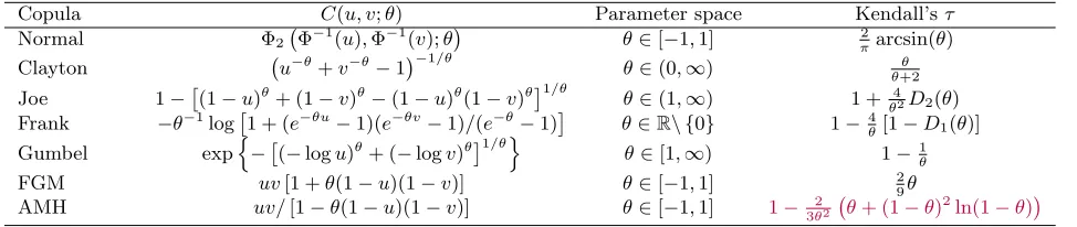
for some two-place functionCwhich is unique, whereθis an association parameter measuring the dependence between the two marginal cdf’s. In the package, the families implemented are normal, Clayton, Joe, Frank, Gumbel, Farlie-Gumbel-Morgenstern (FGM), and Ali-Mikhail-Haq (AMH); these are listed in Table 1. Rotations by 90, 180 and 270 degrees for Clayton, Joe and Gumbel can be obtained using the results reported in Brechmann and Schepsmeier
(2013); these will be available in future releases. As it can be seen from Table 1, θ may be difficult to interpret in some cases. To this end, we can use the Kendall’s τ coefficient which is a measure of association that lies in the customary range [−1,1]. This is generally defined as τ = P((y∗11−y12∗ )(y21∗ −y∗22)>0)−P((y11∗ −y∗12)(y∗21−y22∗ )<0) for independent pairs (y∗1j, y2∗j),j= 1,2, that are copies of (y1∗, y2∗). For each copula there exists a relation between
θ and τ, as shown in Table 1. Testing the null hypothesis of absence of selection bias is an important issue as if the null hypothesis cannot be rejected then joint estimation of the two model equations can be avoided and consistent estimates for the parameters of the equation of interest can be obtained using a univariate equation model. In the context of the copula regression spline sample selection model, the absence of sample selection bias is equivalent
toθ = 0 which in turn is equivalent to the condition that the Kendall’s τ coefficient equals
0. Thus the null hypothesis can, for instance, be tested by checking whether the confidence
interval for the Kendall’s τ includes 0. The problem of testing for sample selection bias is
further addressed in Section4.3. For a comprehensive introduction to the theory of copulas
and their properties see the monographs ofNelsen (2006) andJoe (1997).
Copula likelihood
The log-likelihood function for the sample selection model can be expressed as a sum over two disjoint subsets of the sample: one for the observations with a missing value of the response of interest and the other for the remaining observations. In the first case, the likelihood for the ith observation takes the simple form of P(y
1i = 0), which is equivalent
to F1i(0). In the second case, the joint likelihood can be expressed, using a
multiplica-tion rule, as P(y∗1i > 0)f2|1,i(y2i|y∗1i > 0), where f2|1,i denotes the probability density
func-tion of y∗
2i given y∗1i > 0. After substituting the conditional density f2|1,i(y2i|y∗1i > 0) by
1
P(y∗
1i>0) ∂
∂y2 (F2i(y2)−Fi(0, y2))
y2→y2i, we obtain the log-likelihood
ℓ=
n
X
i=1
(1−y1i) logF1i(0) +y1ilog
f2i(y2i)− ∂ ∂y2
Fi(0, y2)
y2→y2i
.
Using (1), we then have
ℓ=
n
X
i=1
{(1−y1i) logF1i(0) +y1ilog (f2i(y2i) (1−zi))}, (2)
where zi = ∂v∂ C(F1i(0), v;θ)
v→F2i(y2i). The normality of margins implies that F1i(0) =
Φ(−µ1i) andf2i(y2i) =σ−1φ (y2i−µ2i)σ−1, where Φ andφare used throughout to denote
Copula C(u, v;θ) Parameter space Kendall’sτ
Normal Φ2 Φ−1(u),Φ−1(v);θ θ∈[−1,1] 2πarcsin(θ)
Clayton u−θ+v−θ−1−1/θ
θ∈(0,∞) θ
θ+2
Joe 1−
(1−u)θ+ (1−v)θ−(1−u)θ(1−v)θ1/θ
θ∈(1,∞) 1 + 4
θ2D2(θ)
Frank −θ−1log
1 + (e−θu−1)(e−θv−1)/(e−θ−1)
θ∈R\ {0} 1−4θ[1−D1(θ)]
Gumbel expn−
(−logu)θ+ (−logv)θ1/θo
θ∈[1,∞) 1−1
θ
FGM uv[1 +θ(1−u)(1−v)] θ∈[−1,1] 2
9θ
AMH uv/[1−θ(1−u)(1−v)] θ∈[−1,1] 1−3θ22 θ+ (1−θ)
[image:7.595.79.566.109.212.2]2ln(1−θ)
Table 1: Families of copulas implemented in SemiParSampleSel, with corresponding pa-rameter range of the association papa-rameter θ and relation between Kendall’s τ and θ. Φ2(·,·;θ) denotes the cumulative distribution function of a standard bivariate normal
dis-tribution with correlation coefficient θ. D1(θ) = 1θR0θ exp(tt)−1dt is the Debye function and
D2(θ) =R01tlog(t)(1−t)
2(1−θ)
θ dt.
Linear predictor specification
We assume that the expected values µ1i and µ2i of variables y∗1i and y∗2i, respectively, are
linked with the predictors, i.e., µ1i = η1i and µ2i = η2i, where the linear predictor of the
selection equation can be written as
η1i =uT1iα1+
K1
X
k1=1
s1k1(z1k1i), i= 1, . . . n, (3)
and that of the outcome equation as
η2i=uT2iα2+
K2
X
k2=1
s2k2(z2k2i), i∈ {j: y1j = 1}, (4)
where vectoruT1i= (1, u12i, . . . , u1P1i) is theithrow ofU1= (u11, . . . ,u1n)
T, then×P
1 model
matrix containingP1 parametric model components (e.g., intercept, dummy and categorical
variables), α1 is a parameter vector, and thes1k1 are unknown smooth functions of the K1
continuous covariates z1k1i. Our implementation supports varying coefficients’ models,
ob-tained by multiplying one or more smooth terms by some predictor(s) (Hastie and Tibshirani 1993), and smooth functions of two or more (e.g., spatial) covariates as described in Wood
(2006). Similarly, uT2i = (1, u22i, . . . , u2P2i) is the ith row vector of the ns×P2 model
ma-trix U2 = (u21, . . . ,u2ns)
T, where n
s is the size of the selected sample, α2 is a parameter
vector, and the s2k2 are unknown smooth terms of the K2 continuous regressors z2k2i. The
smooth functions are subject to the centering (identifiability) constraint P
isvkv(zvkvi) = 0
for v= 1,2,kv = 1, . . . , Kv (Wood 2006).
The smooth functions are represented using regression splines, where, in the one-dimensional case, a generic sk(zki) is approximated by a linear combination of known spline basis
func-tions, bkj(zki), and regression parameters, βkj, i.e., sk(zki) = PjJ=1k βkjbkj(zki) =βkTBk(zki),
where Jk is the number of spline bases used to represent sk, Bk(zki) is the ith vector of
{bk1(zki), bk2(zki), . . . , bkJk(zki)}
T, and β
k is the corresponding parameter vector. The
sub-script indicating which equation each smooth component belongs to has been suppressed for simplicity. Calculating Bk(zki) for each i yields Jk curves (encompassing different degrees
of complexity) which multiplied by some real valued parameter vector βk and then summed will give a (linear or non-linear) estimate for sk(zk) (see, for instance, Marra and Radice
(2010) for a more detailed overview). Basis functions should be chosen to have convenient mathematical and numerical properties. B-splines, cubic regression and low rank thin plate regression splines are supported in our implementation (see Wood (2006) for full details on these spline bases). The cases of smooths of more than one variable and of varying-coefficient smooth functions follow a similar construction. For instance, in the case of a smooth of two variables z1i and z2i we would have s12(z1i, z2i) = PJj=112 β12jb12j(z1i, z2i), where the
spec-ification of the basis functions depends again on the kind of spline chosen (Wood 2006). Linear predictors (3) and (4) can, therefore, be written as ηvi = uviTαv +BTviβv, where
BTvi =
Bv1(zv1i)T, . . . ,BvKv(zvKvi)T and βTv = (βTv1, . . . ,βTvKv), for v = 1,2. In principle,
the parameters of the sample selection model are identified even if the same regressors appear in both linear predictors (e.g.,Wiesenfarth and Kneib 2010). However, better estimation re-sults are generally obtained when the set of regressors in the selection equation contains at least one or more regressors (usually known as exclusion restrictions) that are not included in the outcome equation (e.g.,Marra and Radice 2013).
2.2. Estimation approach
Denote the log-likelihood function as ℓ(δ), where δT= (δ1T,δ2T, σ, θ) andδvT= (αTv,βTv), for
v = 1,2. Given the flexible structure of the linear predictors considered here, unpenalized estimation can result in smooth term estimates that are too rough to produce practically useful results. This issue is dealt with by using the penalty termP2
v=1
PKv
kv=1λvkv
R
s′′vkv(zvkv)
2dz
vkv
which measures the (typically, second-order) roughness of the smooth terms in the model. For a smooth of two variables generically written as s12(z1, z2) and represented using thin plate
regression splines the integral would look like R R ∂2s12
∂z2 1
2
+ 2 ∂2s12
∂z1∂z2
2
+∂2z12
∂z2 2
2
dz1dz2,
where the subscripts have been dropped to avoid clutter. Theλvkv are smoothing parameters
controlling the trade-off between fit and smoothness. Since regression splines are linear in their model parameters, the overall penalty can be written asβTSλβ where βT= (β1T,β2T), Sλ = P2v=1PKkvv=1λvkvSvkv and the Svkv are positive semi-definite known square matrices
expanded with zeros everywhere except for the elements which correspond to the coefficients of the vkth
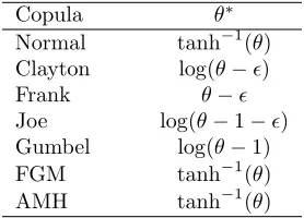
v smooth term. Because of the restrictions on the values that θ can take, we use a
proper transformation of it,θ∗, in order to avoid the use of a constraint when estimating this parameter (see Table2for the list of transformations used). Similarly, since σ can only take positive real values, we useσ∗= log(σ). So, in optimization, we useδT
∗ = (δ1T,δ2T, σ∗, θ∗)∈Rp,
wherepis the total number of parameters. Therefore, the function to maximize is
ℓp(δ∗) =ℓ(δ∗)− 1 2β
TS
λβ. (5)
Given a parameter vector value for ˆλT= (ˆλ1k1, . . . ,λˆ1K1,λˆ2k2, . . . ,λˆ2K2), we seek to maximize
(5). The issues with this maximization problem are thatℓp(δ∗) is not globally concave and the
penalized Hessian may be non-positive definite on some occasions (Toomet and Henningsen
for example, non-concave and/or exhibit regions that are close to flat (Nocedal and Wright
2006, Chapter 4). Let a be an iteration index. Intuitively speaking, line search methods
choose a direction to move from, say, ma to ma+1 and find the distance along that direction
which gives the best improvement in the objective function. If the function is, for instance,
non-convex or has long plateaus, the optimizer may search far away from ma but choose an
ma+1 that is close to ma and that offers marginal improvement in the objective function.
In some cases, the function will be evaluated so far away from ma that it will not be finite
and the algorithm will fail. Trust region methods choose a maximum distance for the move
from ma to ma+1, defining a “trust region” around ma that has a radius of that maximum
distance, and then let a candidate for mt+1 be the minimum of a quadratic approximation
of the objective function. Since points outside of the trust region are not considered, the algorithm never runs too far and/or too fast from the current iteration. The trust region is shrunken if the proposed point in the region is worse/not better than the current point. The new problem with smaller region is then solved. If a point close to the boundary of the trust region is accepted and it gives a large enough improvement in the function then the region for the next iteration is expanded. If a point along a search path causes the objective function to be undefined or indeterminate, most implementations of line search methods will fail and user
intervention is required. In a trust region approach, the search for mt+1 is always a solution
to the trust region problem; if the function at the proposed mt+1 is not finite or not better
than the value at mt, then the proposal is rejected and the trust region shrunken. Finally, a
line search approach requires repeated estimation of the objective function, while trust region methods evaluate the objective function only after solving the trust region problem. Hence, trust region methods can be considerably faster when the objective function is expensive to
compute. Full details can be found in (Nocedal and Wright 2006, Chapter 4).
In practice, we adopt a trust region Newton method (Nocedal and Wright 2006, Chapter 4) which, in our case, solves the problem
min p
˘
ℓp(δ∗[a])def= −
ℓp(δ∗[a]) +pT(g[a]−S∗λˆδˆ [a]) +1
2p
T(H[a]−S∗
ˆ λ)p
so that kpk ≤r[a],
δ∗[a+1] = arg min p
˘
ℓp(δ∗[a]) +δ∗[a],
where k · kdenotes the Euclidean norm andr[a] represents the radius of the trust region. S∗λˆ is the overall block-diagonal penalty matrix which is made up of ˆλvkvSvkv and 0components.
After dropping the iteration index, the score vector g is defined by two subvectors g1 =
∂ℓ(δ∗)/∂δ1 and g2 = ∂ℓ(δ∗)/∂δ2 and two scalars g3 = ∂ℓ(δ∗)/∂σ∗ and g4 = ∂ℓ(δ∗)/∂θ∗, while the Hessian matrix has a 4×4 matrix block structure with (r, h)th element Hr,h =
∂2ℓ(δ∗)/∂δr∂δTh,r, h= 1, . . . ,4, where δ3 =σ∗ and δ4 =θ∗. The expressions of g and Hfor
all copulas are given in Appendix A; these have been derived analytically and verified using numerical derivatives.
At each iteration of the algorithm, ˘ℓp(δ[∗a]) is minimized subject to the constraint that the solution falls within a trust region with radiusr[a]. The proposed solution is then accepted or
Copula θ∗ Normal tanh−1(θ)
Clayton log(θ−ǫ)
Frank θ−ǫ
Joe log(θ−1−ǫ) Gumbel log(θ−1) FGM tanh−1(θ)
[image:10.595.232.371.108.208.2]AMH tanh−1(θ)
Table 2: Transformations,θ∗, of the dependence parameter,θ, used in optimization. Quantity
ǫ is set to the machine smallest positive floating-point number multiplied by 106 and is used
to ensure that the dependence parameters lie in the ranges reported in Table 1.
Smoothing parameter estimation
Multiple smoothing parameter estimation by direct grid search optimization of, for instance, a prediction error criterion can be computationally expensive, especially if the model has more than one smooth term per equation. This section briefly describes the automatic approach employed by Marra and Radice (2013) to estimate λ. Note that joint estimation of δ∗ and
λ via maximization of (5) would clearly lead to overfitting since the highest value for ℓp(δ∗) would be obtained whenλ=0. Parameter vector ˆλ is the solution to the problem
minimize 1
n∗k √
W(z−Xδ∗)k2−1 + 2
n∗
tr(Aλ) w.r.t. λ, (6)
where √W is a weight non-diagonal matrix square root, zi is the 4-dimensional vector
zi=Xiδ∗[a]+W−i 1di,di={∂ℓ(δ∗)i/∂η1i, ∂ℓ(δ∗)i/∂η2i, ∂ℓ(δ∗)i/∂η3i, ∂ℓ(δ∗)i/∂η4i}T,η3i=σ∗, η4i = θ∗, Wi is a 4×4 matrix with (r, h)th element (Wi)rh = −∂2ℓ(δ∗)i/∂ηri∂ηhi, r, h =
1, . . . ,4,Xi= diag
uT1i,BT1i, uT2i,BT2i,1,1 ,n∗ = 4n,Aλ=X(XTWX+S∗λ)−1XTW is
the hat matrix, and tr(Aλ) the estimated degrees of freedom (edf) of the penalized model.
The iteration index has been dropped to avoid clutter. Note that the working linear model quantities are constructed for a given estimate of δ∗. Iteration (6) will produce an updated estimate forλwhich will then be used to obtain a new parameter vector estimate forδ∗. The two steps, one for δ∗ and the other for λ, are iterated until convergence.
To speed up the algorithm the sparse structure of W is exploited. This allows us to set up the working linear model quantities W−1d, √Wz and √WX in O(n∗(m+ 2)) rather than
O(n2∗(m+ 2)) operations, where m is the number of columns of X. Furthermore, since σ∗
and θ∗ are not penalized, the working linear model is constructed for fixed values of these two parameters. In this way, the computational load and storage demand of the algorithm is reduced considerably since in this casen∗ = 2. Theleapfrog algorithm described in Appendix C of Marra and Radice (2013) is employed to achieved this.
2.3. Confidence intervals, variable selection and model selection
of a regression spline sample selection model can be constructed using
δ∗|y∽˙N( ˆδ∗,Vδ∗), (7)
where y refers to the response vectors, ˆδ∗ is an estimate of δ∗ and Vδ∗ = (−H+S∗λˆ)−1.
The structure of Vδ∗ is such that it includes both a bias and variance component in a
fre-quentist sense, which is why such intervals exhibit close to nominal coverage probabilities (Marra and Wood 2012). Given (7), confidence intervals for linear and non-linear functions of the model parameters can be easily obtained. For instance, for a generic ˆsk(zki) these can
be obtained using
ˆ
sk(zki) ˙∽N(sk(zki),Bk(zki)TVδ
∗kBk(zki)), (8)
whereVδ∗k is the submatrix ofVδ∗ corresponding to the regression spline parameters
associ-ated with kth function. Intervals for non-linear functions of the estimated model coefficients (i.e., σ, θ and Kendall’s τ) can be conveniently obtained by simulation from the posterior distribution of δ∗. As for the parametric model components, using (7) is equivalent to using classic likelihood results because such terms are not penalized.
Result (8) can be used to find intervals forsk(zki) for eachkand ibut cannot be used to test
whether smooth terms are equal to zero (e.g., Ruppert, Wand, and Carroll 2003, Chapter
6). For this purpose, p-values or shrinkage methods may be employed. To test smooth components for equality to zero we use the results by Wood(2013). Define ˆsk =Bk(zk) ˆβk,
where Bk(zk) denotes a full column rank matrix and zk = (zk1, zk2, . . . , zkn)T, and Vsk =
Bk(zk)Vδ
∗kBk(zk)
T. It is then possible to obtain approximate p-values for testing smooth
components for equality to zero based on
Trk = ˆs
T
kVsrkk−ˆsk∽˙χ
2
rk,
where Vrk−
sk is the rank rk Moore-Penrose pseudoinverse of Vsk. Parameter rk is selected
using the established notion of edf used in (6). Because edf is not an integer, it can be rounded as follows (Wood 2013)
rk=
(
floor(edfk) if edfk<floor(edfk) + 0.05
floor(edfk) + 1 otherwise
,
which proved effective in semiparametric bivariate probit models (Marra 2013).
As an alternative, the shrinkage single penalty approach presented inMarra and Wood(2011) can be adopted. Specifically, the generic second-order smoothing penalty matrix Sk can be
decomposed as UkΛkUTk, whereUk is an eigenvector matrix associated with the kth smooth
function, and ΛK the corresponding diagonal eigenvalue matrix. Because a part of the spline
basis deals with the penalty null space, Λk contains zero eigenvalues. So even if λk goes to
infinity the smooth term of a nuisance variable may still be estimated as non-zero, because the function component in the null space (i.e., the linear term) is unpenalized. This can be fixed by replacing Λk with ˜Λk, where the latter is the same as the former except that the
zero eigenvalues are set to a small proportion, typically 0.1, of the smallest strictly positive eigenvalue of Sk. This forces the eigenvalues of the new penalty matrix, ˜Sk, associated with
Copula models with a single dependence parameter can be thought of as non-nested models. As suggested byZimmer and Trivedi(2006) among others, one approach for choosing between copula models is to use either the Akaike or (Schwarz) Bayesian information criterion (AIC
andBIC, respectively). In our case,AIC =−2ℓ( ˆδ∗) + 2edf and BIC =−2ℓ( ˆδ∗) + log(n)edf, where the log-likelihood is evaluated at the penalized parameter estimates andedf = tr( ˆAλˆ).
2.4. Numerical considerations
As explained in Section 2.2, a trust region Newton algorithm is a more reliable choice to estimate the model parameters. As for the initial values, they are provided by using an extension of the Heckman (1979) procedure detailed in Appendix B of Marra and Radice
(2013). The adopted approach proved to be fast and reliable in most cases, with occasional convergence failure for small values ofn and ns.
As the analytical expressions for g and H of the copula log-likelihood functions are very
complicated, numerical issues may be encountered in some cases when certain quantities take values which lie nearby their boundaries. Firstly, this may occur when the dependence between the margins is very strong or very weak, i.e., when θ takes extreme values (for example, association tending to 1 implies θ → ∞ for a number of copulas). This leads to expressions which are equal to Inf during the numerical evaluations, especially the Frank copula where the exponential transformation of θappears in the expressions for the gradient and Hessian. Secondly, data points which lie in the tails ofF1i andF2i will lead to their values
equal to 0 or 1. Also, the value of zi appearing in log-likelihood (2) may be approximately
equal to 1, hence producing -Inf. These numerical problems are dealt with by truncating the values of F1i, F2i, f2i and zi to the interval (ε,1−ε) with ε = 10−10. Moreover, the
ratioφ(x)/Φ(x) appearing in the expressions forg andHis defined using the approximation
φ(x)/Φ(x)∼ −x forx <−35 in order to avoidNaN.
If a given model cannot be fitted due to numerical issues then the user receives the message
Ill-conditioned task. It is worth noting that numerical problems that arise when fitting a model may be also a hint that the chosen model is not appropriate to fit the data at hand.
3. Overview of the package
The SemiParSampleSel package is available from the Comprehensive R Archive Network
(CRAN) at http://cran.r-project.org/web/packages/SemiParSampleSel/index.html. The package depends onmagic(Hankin 2005), mgcv(Wood 2006),trust (Geyer 2013), mvt-norm (Genz and Bretz 2009), Matrix (Bates and Maechler 2014) and copula (Yan 2007). The main function in SemiParSampleSel is SemiParSampleSel(), which fits copula regres-sion spline sample selection models as described in the previous section. The function can be called using the following syntax:
SemiParSampleSel(formula.eq1, formula.eq2, data = list(), BivD = "N", margins = c("N", "N"), gamma = 1, ...)
y.sel ~ as.factor(x1) + s(x2, bs = "cr", k = 10, m = 2) + s(x3, x4) + ...,
where y.sel represents the binary selection variable, x1 is a categorical predictor, and the
s terms are used to specify smooth functions of the continuous predictors x2, x3 and x4. Argument bs specifies the spline basis; possible choices includecr (cubic regression spline),
cs(shrinkage version ofcr),tp(thin plate regression spline) andts(shrinkage version oftp). Bivariate smoothing, e.g., s(x3, x4), is achieved usingbs = "tp". kis the basis dimension (default is 10) and m the order of the penalty (default is 2). More details and options on smooth term specification can be found in the documentation of mgcv. SemiParSampleSel
does not currently support the use of tensor product smooths.
Optional arguments of the functionSemiParSampleSel include data which is a data frame, list or environment containing the variables in the model, and gamma which is an inflation factor for the model degrees of freedom used in the smoothing step. Smoother models can be obtained setting this parameter to a value greater than 1. In our experience, gamma = 1.4typically achieves this; this was also found byKim and Gu(2004) in a different context. The type of bivariate copula linking the two model equations can be specified throughBivD. Possible choices are "N", "C", "J", "FGM", "F", "AMH" and "G" which stand for bivariate normal, Clayton, Joe, Farlie-Gumbel-Morgenstern, Frank, Ali-Mikhail-Haq and Gumbel. The argumentmarginsspecifies the marginal distributions of the selection and outcome equations, given in the form of a two-dimensional vector which is equal to c("N","N") for normal margins. Details on all the other arguments, including starting value and control options, and the fitted-object list that the function returns can be found in (Marra et al. 2014). Other available functions are:
plot(x, eq, pages = 0, scale = -1, shade = FALSE, seWithMean = FALSE, ...). This function takes a fitted objectxas produced bySemiParSampleSel()and plots the component smooth functions that make it up on the scale of the linear predictor. eq
denotes the equation from which smooth terms should be considered for printing,pages
is the number of pages over which to produce the plots (e.g., ifpages = 1then all terms will be plotted on one page), and scaleis the y-axis scale to use for each plot (scale = 0gives a different axis for each plot). Ifshadeis set toTRUEthen shaded regions as con-fidence bands for smooth terms are produced. Of interest is the argument seWithMean
which indicates whether the component smooth should be shown with confidence in-tervals that include the uncertainty about the overall mean. Marra and Wood (2012) showed that seWithMean = TRUE results in intervals with better nominal frequentist coverage probabilities. This function is based on plot.gam() in mgcv to which the reader is referred for full details.
predict(object, eq, ...). This function takes a fitted SemiParSampleSel object and produces predictions for a new set of values of the model covariates or the original values used for the model fit. Standard errors of predictions can be produced. These are based on the posterior distribution of the model coefficients. This function is based on predict.gam()inmgcv.
estimated model parameters, which are used to calculate ‘confidence’ intervals for σ,θ
and Kendall’sτ, for instance. s.methis the matrix decomposition used to determine the matrix root of the covariance matrix (see the documentation ofmvtnormfor further de-tails). prob.levis the probability of the left and right tails of the posterior distribution used for interval calculations. The object list returned includes, for instance, summary tables for the selection and outcome equations for the parametric and nonparametric components, and the estimated standard deviation and association coefficient.
ss.checks(x)which produces some diagnostic information about the fitting procedure for a SemiParSampleSel object.
These functions will be illustrated in Section 5.
4. Simulations
In this section, we conduct a Monte Carlo simulation study to evaluate the empirical effec-tiveness of the copula regression spline sample selection models implemented in the package. For convenience, all the tables and figures of results are given in Appendix B.
As inMarra and Radice(2013), the sampling experiments were based on the equations
η1i =α11+α12ui+s11(z1i) +s12(z2i) η2i =α21+α22ui+s21(z1i)
, (9)
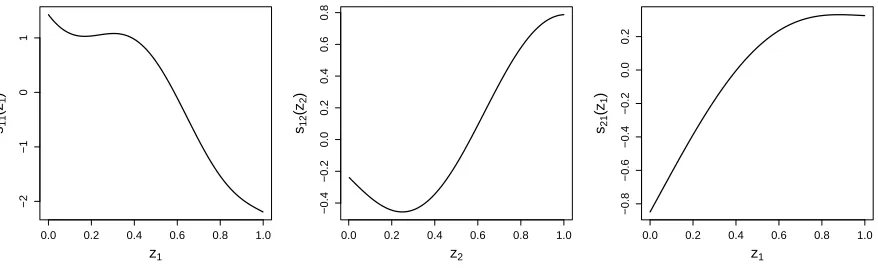
wherey1iandy2iwere determined as described in Section2.1. The test functions are displayed
in Figure 1 and are defined as s11(z1i) = −0.7
4z1i+ 2.5z12i+ 0.7 sin(5z1i) + cos(7.5z1i) , s12(z2i) = −0.4{−0.3−1.6z2i+ sin(5z2i)}, and s21(z1i) = 0.6{exp(z1i) + sin(2.9z1i)}.
Pa-rameter vector (α12, α21, α22) andσ were set to (2.5,−0.68,−1.5) and 1. Binary values fory1i
were generated so that approximately 50% of the total number of observations were selected to fit the outcome equation; this was achieved by setting α11 to 0.58. Regressorsui,z1i and z2i were generated as three uniform covariates on (0,1) with correlation approximately equal
to 0.5. This was achieved usingrmvnorm()inmvtnorm, generating standardized multivariate random draws with correlation 0.5 and then applyingpnorm()(e.g.,Marra and Radice 2013). Regressorui was eventually dichotomized usinground(). As joint distribution of (y1∗i, y2i)ni=1
the following copulas were considered: normal, Clayton, Joe, FGM, AMH, Frank and Gum-bel, each with normal margins. The sample sizenwas set to 1000. For each copula, different values of the association parameter were considered:
normal copula: θ= 0.16 (τ = 0.1), θ= 0.71 (τ = 0.5), θ= 0.89 (τ = 0.7),
Clayton copula: θ= 0.22 (τ = 0.1),θ= 2 (τ = 0.5),θ= 57 (τ = 0.7),
Joe copula: θ= 1.31 (τ = 0.15),θ= 2.86 (τ = 0.5),θ= 6.78 (τ = 0.75),
FGM copula: θ=−0.9 (τ =−0.2),θ= 0.68 (τ = 0.15),
AMH copula: θ=−0.62 (τ =−0.12), θ= 0.4 (τ = 0.1), θ= 0.9 (τ = 0.28),
Gumbel copula: θ= 1.25 (τ = 0.2),θ= 2 (τ = 0.5),θ= 5 (τ = 0.8).
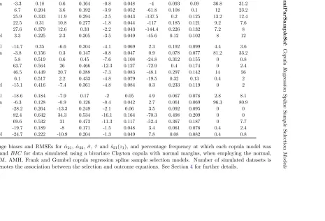
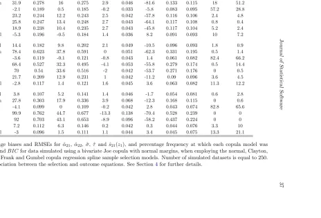
In Tables 4 -10 the association parameter used to generate the data is expressed in terms of Kendall’sτ coefficient. For each combination of parameter settings, the number of simulated datasets was set to 250. We also explored the performance of the models in the absence of an exclusion restriction as detailed in Section4.2.
0.0 0.2 0.4 0.6 0.8 1.0
−2
−1
0
1
z1
s11 (z1
)
0.0 0.2 0.4 0.6 0.8 1.0
−0.4
−0.2
0.0
0.2
0.4
0.6
0.8
z2
s12 (z2
)
0.0 0.2 0.4 0.6 0.8 1.0
−0.8
−0.6
−0.4
−0.2
0.0
0.2
z1
s21 (z1
[image:15.595.85.524.205.339.2])
Figure 1: The test functions used in the simulation studies.
4.1. Main results
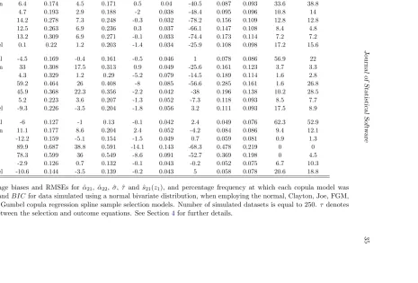
Since the selection equation is not in principle affected by non-random sample selection bias, we focus on the estimation results for the outcome equation only. Tables 4 - 10 report the percentage relative bias and root mean squared error (RMSE) calculated for the estimators of
α21,α22,σ,τ, and the RMSE for that ofs21(z1), calculated as
q
1 200
P200
b=1{sˆ(z1b)−s(z1b)} 2
, based on the estimates for 200 fixed covariate values. The tables also report the percentage frequency at which each copula model was selected byAIC andBIC.
The results presented in the tables show overall that the model employing the true copula achieves the lowest bias and/or RMSE of the estimators of all considered parameters in most cases. We can particularly observe this for data generated using the Clayton copula (see Table 5), where the estimators of α21, α22, σ, τ and s22 obtained from the Clayton model
outperform in terms of bias and RMSE those yielded by the other copula models. Using the right model is particularly important for estimating τ when its true value falls outside the dependence range covered by a given copula, as some of them allow only for a restricted interval of dependence (here, this is the case for AMH and FGM). The results also show that, for data generated using the Frank or normal copulas, both models yield comparably good results, hence reflecting the similarity between these two copulas (see Tables4and9for
τ = 0.7). We observe a similar effect for data generated using the Joe and Gumbel copulas. The findings also suggest that in some cases for small values of τ the choice of the correct copula model does not seem to play an important role in estimation (see Table 4forτ = 0.1, Table 7 and Table 8), and often the Clayton and Gumbel models yield estimators with a relatively low bias and RMSE for such data regardless of the true copula.
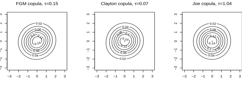
As an example, Figure2 presents contour plots of FGM, Clayton and Joe copulas with nor-mal margins for snor-mall values of the dependence parameter. For those distributions the choice of the correct copula based on an empirical sample is extremely difficult and the selection
criteria appear to select an arbitrary model as can be seen in Table 7. At the same time,
the finite sample performance of the estimators is unaffected by the wrong choice of a copula in those border cases as, again, all copulas tend to the same (normal product) distribution
here. Also, even in this difficult situation, AIC seems to be successful for some copulas (see
Tables 5, 6 and 9). For medium and large values of τ, the true copula model is the most frequent choice with all model selection criteria, withAIC performing much better thanBIC
and achieving a hit rate of more than 90% in some cases (see Table5). It is also worth noting that in general, the accuracy of the choice of the copula improves with the sample size as can be seen in Tables 1 and 2 of supplementary materials where the experiment was repeated for samples of sizen= 3000 andn= 5000 pertaining to bivariate normal distribution. There we can also observe consistency of the estimators when the right copula is chosen. In the case of a wrong copula the estimators are inconsistent.
FGM copula, τ=0.15
0.02
0.04 0.06
0.08 0.1 0.12
0.14
−3 −2 −1 0 1 2 3
−3
−2
−1
0
1
2
3
Clayton copula, τ=0.07
0.02 0.04
0.06
0.08 0.1
0.12 0.14
−3 −2 −1 0 1 2 3
−3
−2
−1
0
1
2
3
Joe copula, τ=1.04
0.02
0.04 0.06
0.08
0.1 0.12
0.14
−3 −2 −1 0 1 2 3
−3
−2
−1
0
1
2
[image:16.595.107.499.332.471.2]3
Figure 2: Contour plots of FGM, Clayton and Joe copulas with normal margins for small values of the dependence parameter.
4.2. Absence of an exclusion restriction
Sometimes the same regressors have to be used in both selection and outcome equations as an exclusion restriction is not available. To investigate the performance of the copula sample selection models in this situation, the simulation study described above was repeated for the case in which system (9) did not includes12(z2i). The sampling experiments were based on
η1i=α11+α12ui+s11(z1i) η2i=α21+α22ui+s21(z1i)
, (10)
where functionss11 and s21 and parameters α11,α12,α21,α22 were the same as in Section4
and the predictorsui and z1i were generated in the same way.
simulated data were based on the equations
η1i=α11+α12ui+s21(z1i) η2i=α21+α22ui+s21(z1i)
. (11)
Figures5and6demonstrate the influence of the lack of exclusion restriction on the estimators of the model parameters in terms of their mean squared error and bias, for a choice of copulas: normal, Clayton, Joe and FGM. The solid lines correspond to root mean squared errors of the estimators ˆα21, ˆα22, ˆσ, ˆτ and the smooth function ˆs21(upper panels) and absolute values
of percentage bias of estimators ˆα21, ˆα22, ˆσ and ˆτ (lower panels) for model (10) without the
exclusion restriction. The corresponding lines for model (9) in which the selection equation contains an additional term s12(z2) are added for comparison as dotted lines. Analogically,
Figures7and8demonstrate the influence of the lack of exclusion restriction on the estimators for model (11) in comparison to model (9).
We observe that the quality of the estimator ˆσis practically unaffected by the lack of exclusion restriction for both scenarios considered in terms of root mean squared error and bias. For the remaining parameters, we observe that removings12(z2) from the selection equation increases
the bias and RMSE of the estimators in most of the cases considered. We also observe a larger variance and more cases of lack of convergence when the exclusion restriction is not available. The lack of exclusion restriction leads to particularly unstable estimators of the Kendall’s τ in terms of the relative bias in cases where this parameter is close to zero, as can be seen in figures 5a) and6b) where the relative percentage bias exceeds 160% and 110%, respectively, while the RMSEs of ˆτ in those cases do not indicate any particularly bad performance. The above values of relative bias imply however that the average estimated values of τ equal approximately −0.06 and −0.018, respectively, which in turn has a major importance while testing the absence of sample selection bias as it affects the size and power of the test. This issue is further discussed in section4.3. However, for scenario (10) the influence of the lack of exclusion restriction is usually much less significant than for the more difficult scenario (11). Moreover, in some cases the differences between the RMSEs of the model parameters for the cases with and without the exclusion restriction are rather negligible (see Figure 5 b) and Figure6 a)).
4.3. Testing the absence of sample selection bias
The key issue while fitting a sample selection model is testing the null hypothesis of absence of
selection bias. If the variablesy∗
1i and y∗2i are correlated then the sample selection bias occurs
and it is necessary to consider both outcome equation and selection equation together with the dependence structure between the two of them while estimating the model. Otherwise, the model can be much simplified by dropping the selection equation (and consequently the copula function) from the analysis.
In general, the approach to testing for sample selection bias relies heavily on the specific
sample selection model assumed. In the Heckman’s two step procedure (Heckman (1979))
sample selection bias is tested using the t-test related with the significance of the omitted
variable. Dubin and Rivers (1989) considered likelihood ratio, Wald and Lagrange multiplier
tests in the context of a censored probit model. Moreover,Vella(1992) proposed a conditional
moment test.
bias can be based on the dependence parameterθas absence of sample selection bias is
equiv-alent to the condition θ= 0. However, because of the restrictions on the values of the copula
association parameters, the use of classic testing approaches may yield unreliable results in
some copula cases. As a practical alternative, the Kendall’s τ coefficient can be employed.
Hence the null hypothesis can be tested by checking whether the confidence interval for τ
includes 0. In this section, results of a Monte-Carlo study of the finite-sample performance of such approach are presented.
For data sets generated using the equations (9), the empirical size of the test for absence of selectivity bias has been calculated based on 99%, 95% and 90% confidence intervals for the parameter τ. As before, for every data set different copulas were considered while fitting the spline sample selection models (normal, FGM, AMH, Frank and Gumbel). The Clayton and Joe copulas are not considered in the study as they allow only strictly positive dependence implying that the size of the test always equals 1 in this case. The results of the Monte Carlo simulations based on 250 repetitions are presented in table 11. The smallest values of the empirical sizeαcan be observed while using copulas FGM and AMH, which can be intuitively explained by the fact that both of those copulas allow very restricted range of the parameterτ (τ ∈[−2/9,2/9] for FGM and τ ∈[−0.1817,1/3] for AMH) which implies that models based on FGM and AMH copulas are well suited for data with very weak dependence. Among the three remaining copulas, which allow the full range of dependence, i.e. τ ∈ (−1,1), Frank copula performs the best achieving the empirical size of the test very close to the theoretical value forn= 5000. The poorest performance occurs in the case of Gumbel copula for which the empirical size converges to the theoretical value at a much slower rate, as the sample size increases.
Tables12 and13present the empirical size for the sample selection bias test for data without exclusion restriction, generated using the equations (10) and (11), respectively. In both cases, a negative influence of lack of an the exclusion restriction can be observed as the values of empirical sizes are larger than those presented in table 11 where the exclusion restriction is used. Moreover, the effect of lack of exclusion restriction is more severe for data generated using equations (11) where the variablez1 enters both, the selection and the
outcome equations, in the same functional form. However, in Tables 12 and 13 the same tendency regarding to the comparison between different copulas can be observed with FGM and AMH achieving the smallest empirical sizes and Gumbel copula displaying the worst performance.
Moreover, a study of empirical power of the test for sample selection bias has been conducted,
with results reported in Tables 14-15. As expected, the power of all tests drops when the
dependence parameter is close to 0, i.e., when the selection and outcome equations are close to independence. In this difficult scenario, using Gumbel copula leads to the most powerful tests. A particularly poor performance can be observed when fitting the FGM and AMH
copulas. Those are the copulas allowing very limited scope of parameter τ which makes
them perform poorly not only in the proximity of the null hypothesis but also when a strong dependence holds. For the three remaining copulas, a very good performance can be observed
when the coefficient τ equals at least 0.5 as the power usually exceeds the level of 97% in
Tables16-19present powers of the test for sample selection bias in the absence of an exclusion restriction. In most of the cases considered, the powers of the test are smaller than when the exclusion restriction is present. However, in some cases larger powers also can be observed for data generated using FGM and AMH copulas. Thus the absence of an exclusion restriction appears to affect the testing process more severely when the correlation between the two model equations is moderate or strong.
5. Real data example
The copula regression spline sample selection models presented in this paper are illustrated using data from the RAND Health Insurance Experiment (RHIE) which was a comprehensive study of health care cost, utilization and outcome conducted in the United States between 1974 and 1982 (Newhouse 1999). As explained in the introductory section, the aim was to quantify the relationship between various covariates and annual health expenditures in the population as a whole.
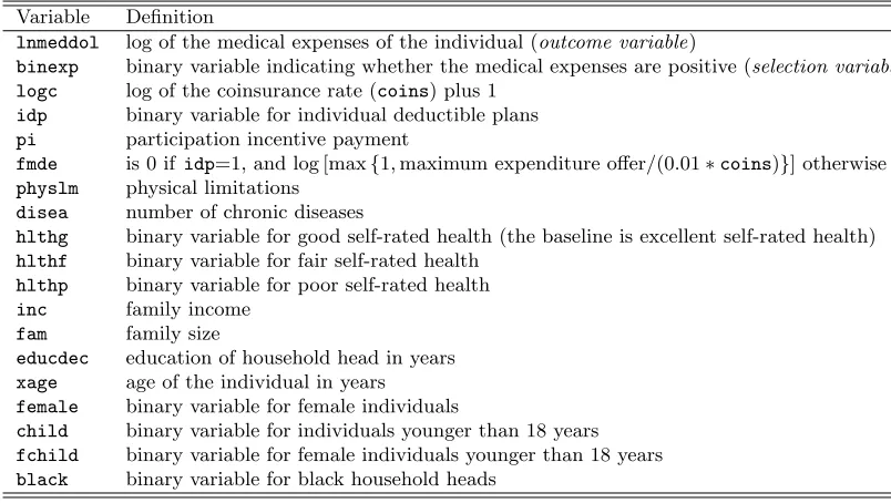
Variable Definition
lnmeddol log of the medical expenses of the individual (outcome variable)
binexp binary variable indicating whether the medical expenses are positive (selection variable) logc log of the coinsurance rate (coins) plus 1
idp binary variable for individual deductible plans
pi participation incentive payment
fmde is 0 if idp=1, and log [max{1,maximum expenditure offer/(0.01∗coins)}] otherwise
physlm physical limitations
disea number of chronic diseases
hlthg binary variable for good self-rated health (the baseline is excellent self-rated health)
hlthf binary variable for fair self-rated health
hlthp binary variable for poor self-rated health
inc family income
fam family size
educdec education of household head in years
xage age of the individual in years
female binary variable for female individuals
child binary variable for individuals younger than 18 years
fchild binary variable for female individuals younger than 18 years
[image:19.595.92.494.334.561.2]black binary variable for black household heads
Table 3: Description of the outcome and selection variables, and of the regressors.
In this context, non-random sample selection arises because the sample consisting of indi-viduals who used health care services differ in important characteristics from the sample of individuals who did not use them. Because some characteristics cannot be observed, tradi-tional regression modeling is likely to deliver inconsistent estimates, hence the need to correct parameter estimates for non-random sample selection. We use the same subsample as in
Cameron and Trivedi (2005, p. 553), and model annual health expenditures. The sample size and number of selected observations are 5574 and 4281. The variables are defined in Table3. Additional information can be found inCameron and Trivedi(2005, Table 20.4) and
Newhouse(1999).
fmde,physlm,disea,hlthg,hlthf,hlthp,female,child,fchildandblackas parametric components, and smooth functions of pi, inc, fam, educdec and xage, represented using thin plate regression splines with basis dimensions equal to 10 and penalties based on second-order derivatives (which are the default options in the package). Specifically, after reading the dataset, called ND, we load the package and specify the selection and outcome equations.
R> library(SemiParSampleSel)
R> SE <- binexp ~ logc + idp + fmde + physlm + disea + hlthg + hlthf +
hlthp + female + child + fchild + black + s(pi) + s(inc) + s(fam) + s(educdec) + s(xage)
R> OE <- lnmeddol ~ logc + idp + fmde + physlm + disea + hlthg + hlthf +
hlthp + female + child + fchild + black + s(pi) + s(inc) + s(fam) + s(educdec) + s(xage)
We then estimate the copula regression spline sample selection models by penalized likelihood, as described in Section 2.2, setting gamma = 1.4to obtain smoother models.
R> out_N <- SemiParSampleSel(SE, OE, data = ND, gamma = 1.4)
R> out_C <- SemiParSampleSel(SE, OE, data = ND, BivD = "C", gamma = 1.4)
R> out_J <- SemiParSampleSel(SE, OE, data = ND, BivD = "J", gamma = 1.4)
R> out_FGM <- SemiParSampleSel(SE, OE, data = ND, BivD = "FGM", gamma = 1.4)
R> out_F <- SemiParSampleSel(SE, OE, data = ND, BivD = "F", gamma = 1.4)
R> out_AMH <- SemiParSampleSel(SE, OE, data = ND, BivD = "AMH", gamma = 1.4)
R> out_G <- SemiParSampleSel(SE, OE, data = ND, BivD = "G", gamma = 1.4)
Given the superior performance ofAIC on BIC shown in the simulation study, we use the
AIC to select a model.
R> AIC_N <- AIC(out_N)
R> AIC_C <- AIC(out_C)
R> AIC_J <- AIC(out_J)
R> AIC_FGM <- AIC(out_FGM)
R> AIC_F <- AIC(out_F)
R> AIC_AMH <- AIC(out_AMH)
R> AIC_G <- AIC(out_G)
R> AIC_N
[1] 20294.88
R> AIC_C
[1] 20298.31
R> AIC_J
R> AIC_FGM
[1] 20287.24
R> AIC_F
[1] 20281.23
R> AIC_AMH
[1] 20282.8
R> AIC_G
[1] 20293.89
The Frank copula model is chosen. Before looking at the results, we check that the algorithm has found a solution.
R> ss.checks(out_F)
Largest absolute gradient value: 2.726033e-07 Information matrix is positive definite
Trust region Newton iterations before smoothing parameter estimation: 6 Smoothing parameter/leapfrog loops: 4
Trust region Newton iterations after smoothing parameter/leapfrog step: 2
We can now look at the results.
R> set.seed(1) R> summary(out_F)
Family: SAMPLE SELECTION Frank Copula with normal margins
SELECTION EQ.: binexp ~ logc + idp + fmde + physlm + disea + hlthg + hlthf + hlthp + female + child + fchild + black + s(pi) + s(inc) +
s(fam) + s(educdec) + s(xage)
hlthg 0.083350 0.044482 1.874 0.060956 . hlthf 0.190734 0.083414 2.287 0.022220 * hlthp 0.590048 0.208658 2.828 0.004687 ** female 0.463019 0.054950 8.426 < 2e-16 *** child 0.252364 0.146261 1.725 0.084449 . fchild -0.457734 0.080554 -5.682 1.33e-08 *** black -0.591727 0.054067 -10.944 < 2e-16 ***
---Signif. codes: 0 *** 0.001 ** 0.01 * 0.05 . 0.1 1
Smooth components approximate significance: edf Est.rank Chi.sq p-value s(pi) 8.035 8 34.022 4.03e-05 *** s(inc) 2.485 3 30.990 8.54e-07 *** s(fam) 1.805 2 2.071 0.355006 s(educdec) 1.623 2 14.962 0.000564 *** s(xage) 6.921 7 51.414 7.62e-09 ***
---Signif. codes: 0 *** 0.001 ** 0.01 * 0.05 . 0.1 1
OUTCOME EQ.: lnmeddol ~ logc + idp + fmde + physlm + disea + hlthg + hlthf + hlthp + female + child + fchild + black + s(pi) + s(inc) +
s(fam) + s(educdec) + s(xage)
Estimate Std. Error z value Pr(>|z|) (Intercept) 4.007309 0.092939 43.118 < 2e-16 *** logc 0.008707 0.033452 0.260 0.794634 idp -0.068785 0.064412 -1.068 0.285574 fmde -0.028829 0.020067 -1.437 0.150831 physlm 0.198391 0.070378 2.819 0.004818 ** disea 0.015770 0.003622 4.354 1.34e-05 *** hlthg 0.142250 0.049331 2.884 0.003932 ** hlthf 0.327870 0.089692 3.656 0.000257 *** hlthp 0.631742 0.174589 3.618 0.000296 *** female 0.214176 0.059725 3.586 0.000336 *** child 0.017721 0.170062 0.104 0.917008 fchild -0.229596 0.091147 -2.519 0.011771 * black -0.024775 0.070988 -0.349 0.727087
---Signif. codes: 0 *** 0.001 ** 0.01 * 0.05 . 0.1 1
s(educdec) 1.966 2 2.436 0.295892 s(xage) 7.084 8 31.027 0.000139 ***
---Signif. codes: 0 *** 0.001 ** 0.01 * 0.05 . 0.1 1
n = 5574 n.sel = 4281 sigma = 1.422(1.386,1.46)
theta = -3.043(-3.942,-2.268) Kendall s Tau = -0.311(-0.384,-0.24) total edf = 66.648
Notice that we set a seed before summary(). This allows us to recover the same results for the confidence intervals of the quantities reported at the bottom of the summary output; recall that intervals for such components are calculated using Bayesian posterior simulation as mentioned in Section 2.3.
As for the selection equation, the results show that all variables, which enter the model parametrically, are statistically significant at the 10% level, except for fmde. The p-values for the smooth terms, calculated as discussed in Section2.3, indicate thatfamdoes not have an impact on the response. Regarding the outcome equation, health status variables (such as physlm and disea) have an effect on annual health expenses, whereas health insurance variables (logc and idp) seem not to determine the medical expenses. The p-values for the estimated smooths indicate thatinc,famandxage are significantly different from zero. The estimate forσ is 1.42 and is significantly different from zero. The estimate for θ is negative and statistically different from zero. Kendall’s Tauis also negative and significantly different from zero. This indicates that the unobserved factors which affect the use of health services also affect medical expenses. The estimated degrees of freedom (total edf) of the penalized model, calculated as described in Section2.2, is 66.648.
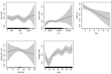
Usingplot(), we produce the smooth function estimates for the outcome equation obtained from the Frank copula model; these are displayed in Figure3.
R> plot(out_F, eq = 2, pages = 1, scale = 0, shade = TRUE, seWithMean = TRUE, cex.axis = 1.6, cex.lab = 1.6)
The shaded regions represent 95% confidence bands calculated from the posterior distribution, as described in Section2.3. The ‘rug plot’, at the bottom of each graph, shows the covariate values. The numbers shown on the y-axis in each plot indicate the estimated degrees of free-dom (edf). Due to the identifiability constraints, the estimated curves are centered around zero. The results forxage and famare consistent with the interpretation that health expen-diture increases non-linearly as people become older, and that individual health expenexpen-diture decreases as family size increases.
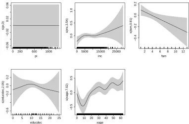
We re-fit the Frank copula regression model by using the shrinkage optionbs = "ts"ins().
R> SE_s <- binexp ~ logc + idp + fmde + physlm + disea + hlthg + hlthf + hlthp + female + child + fchild + black +
s(pi, bs = "ts") + s(inc, bs = "ts") + s(fam, bs = "ts") + s(educdec, bs = "ts") + s(xage, bs = "ts")
s(pi, bs = "ts") + s(inc, bs = "ts") + s(fam, bs = "ts") + s(educdec, bs = "ts") + s(xage, bs = "ts")
R> out_F_s <- SemiParSampleSel(SE_s, OE_s, data = ND, BivD = "F", gamma = 1.4) R> plot(out_F_s, eq = 2, pages = 1, scale = 0, shade = TRUE, seWithMean = TRUE,
cex.axis = 1.6, cex.lab = 1.6)
0 200 600 1000
−0.4
0.0
0.2
0.4
0.6
pi
s(pi,4.08)
0 5000 15000 25000
−0.5
0.0
0.5
1.0
inc
s(inc
,3.65)
2 4 6 8 10 12
−0.6
−0.4
−0.2
0.0
0.2
fam
s(f
am,1)
0 5 10 15 20 25
−0.6
−0.4
−0.2
0.0
0.2
educdec
s(educdec
,1.97)
0 10 20 30 40 50 60
−0.5
0.0
0.5
xage
s(xage
[image:24.595.105.485.214.470.2],7.08)
Figure 3: Smooth function estimates and 95% confidence bands obtained applying the Frank copula regression spline sample selection model on the RAND RHIE dataset described in Section 4.
We obtain the fitted smooth functions depicted in Figure4; regressorpihas been suppressed, whereas the other covariate effects exhibit patterns similar to those reported in Figure3.
Finally, we use predict() to produce a prediction for new values of the model covariates. Specifically, we predict the log of medical expenditure for a typical individual.
R> new_data <- data.frame(logc = median(ND$logc), idp = median(ND$idp),
fmde = median(ND$fmde), physlm = median(ND$physlm), disea = median(ND$disea), hlthg = median(ND$hlthg), hlthf = median(ND$hlthf), hlthp = median(ND$hlthp), female = median(ND$female), child = median(ND$child), fchild = median(ND$fchild), black = median(ND$black), pi = mean(ND$pi), inc = mean(ND$inc), fam = mean(ND$fam), educdec = mean(ND$educdec), xage = mean(ND$xage))
0 200 600 1000
−0.06
−0.02
0.02
0.06
pi
s(pi,0)
0 5000 15000 25000
0.0
0.5
1.0
inc
s(inc
,3.54)
2 4 6 8 10 12
−0.4
−0.2
0.0
0.2
fam
s(f
am,0.81)
0 5 10 15 20 25
−0.6
−0.2
0.0
0.2
educdec
s(educdec
,2.06)
0 10 20 30 40 50 60
−0.5
0.0
0.5
xage
s(xage
[image:25.595.104.486.122.373.2],7.02)
Figure 4: Smooth function estimates and 95% confidence bands obtained applying the Frank copula model with shrinkage option on the RAND RHIE dataset.
1 4.430282
6. Discussion
We introduced flexible continuous response sample selection models and discussed theR
pack-ageSemiParSampleSelwhich implements them. The package can be used to fit models where
the linear predictors are flexibly specified using parametric and non-parametric components, and the dependence between the selection and outcome equations is modeled through the use of copulas. The developments and implementation proposed here extend and complement previous R implementations of sample selection models. Allowing for non-normal bivariate
distributions between the model equations is important since the assumption of bivariate normality is often criticized.
The reader is cautioned that the class of models presented here is not intended to be exhaus-tive; as the majority of the methods, under model misspecification the proposed approach does not provide consistent estimates. For example, if the marginals are non-normal (e.g., they exhibit a heavy-tailed behavior or can be modeled using skewed, contaminated and mix-ture distributions), biased estimates should be expected. The extent of the bias cannot be
predicted a priori and it depends on the application at hand. In light of this,possible
gener-alizations of the methods implemented inSemiParSampleSel are to extend the scope of the marginal distribution for the outcome equation, using for instance the gamma, Poisson and Student-t distributions, and that of the available copulas in the package, using for example the Plackett and rotated copulas. Future research will also concern the development of model checking tools.
Acknowledgments
The first two authors were supported by the Engineering and Physical Sciences Research Council, UK (Grant EP/J006742/1). We are indebted to two anonymous reviewers for their constructive criticism which helped to improve considerably the presentation of the article.
References
Ahn H, Powell JL (1993). “Semiparametric Estimation of Censored Selection Models With a Nonparametric Selection Mechanism.”Econometrics,58, 3–29.
Andrews DWK, Schafgans MMA (1998). “Semiparametric Estimation of the Intercept of a Sample Selection Model.”Review of Economic Studies,65, 497–517.
Bates D, Maechler M (2014). Matrix: Sparse and Dense
Ma-trix Classes and Methods. R package version 1.1-2, URL
http://cran.r-project.org/web/packages/Matrix/index.html.
Bhat CR, Eluru N (2009). “A Copula-Based Approach to Accommodate Residential Self-Selection Effects in Travel behavior modeling.” Transportation Research Part B: Method-ological,43, 749–765.
Brechmann EC, Schepsmeier U (2013). “Modeling Dependence with C- and D-Vine Copulas: The R Package CDVine.” Journal of Statistical Software, 52(3), 1–27. ISSN 1548-7660. URLhttp://www.jstatsoft.org/v52/i03.
Cameron A, Trivedi P (2005). Microeconometrics: Methods and Applications. Cambridge University Press, New York.
Chen S, Zhou Y (2010). “Semiparametric and Nonparametric Estimation of Sample Selection Models under Symmetry.”Journal of Econometrics,157, 143–150.