IJPSR (2018), Volume 9, Issue 4 (Review Article)
Received on 18 July, 2017; received in revised form, 24 October, 2017; accepted, 17 November, 2017; published 01 April, 2018
A BRIEF OVERVIEW ON MOLECULAR DYNAMICS SIMULATION OF BIOMOLECULAR SYSTEM: PROCEDURE, ALGORITHMS AND APPLICATIONS
Saurabh Gupta and Pritish Kumar Varadwaj*
Department of Applied Sciences, Indian Institute of Information Technology, Allahabad - 211012, Uttar Pradesh, India.
ABSTRACT: Molecular Dynamics (MD) Simulation provides the details explanation of the atomic and molecular interactions that directed by macroscopic and microscopic behaviors of the various systems. This review provides a brief do-how about the theory, procedure, algorithm, and uses of molecular dynamic simulations in different bimolecular systems. An in-depth analysis of different prospects of MD simulation viz. procedure of MD simulation, force fields, energy minimization and integration algorithms, concept of ensembles and thermostats with a list of associated software briefly explained. At last discussion of various applications of MD simulation using some recent works, indicates the potential contribution of MD in biological research.
INTRODUCTION: In late 50’s, Alder and Wainwright, first time introduced the concept of Molecular Dynamics (MD) to find out the interactions of hard spheres by utilizing Monte Carlo Simulation. This concept further used explored important behavioral insight of simple liquids 1, 2. In 1964, Rahman carried out another simulation using a realistic potential for liquid Argon 3. Further, in 1974, Rahman and Stillinger performed the first ever molecular dynamics simulation of a realistic system using liquid water solvent model 4. Mc-Cammon et al., in 1977 for the first time performed a simulation of the Bovine Pancreatic Trypsin Inhibitor (BPTI).
QUICK RESPONSE CODE
DOI:
10.13040/IJPSR.0975-8232.9(4).1333-50
Article can be accessed online on:
www.ijpsr.com
DOI link: http://dx.doi.org/10.13040/IJPSR.0975-8232.9(4).1333-50
These days MD simulations are being profoundly used for various purposes such as simulation of dynamic surface exploration of proteins, study of various protein macromolecular complexes (e.g. protein-protein, protein-DNA, and protein-ligand interactions) and lipid systems. The MD addresses several of issues such as thermodynamics of protein-ligand complex, proteins folding, umbrella sampling of protein, free energy calculation of molecule, membrane protein simulation and study of ion transport etc. 5.
The different simulation methods having searching algorithms and force field parameterizations enabled the users to use different options according to their bimolecular system. These techniques use the principle of classical mechanics, molecular mechanics, and quantum mechanics; for understanding various biochemical systems viz. enzymatic reactions, chemical pathways, and thermodynamic study. In addition, simulation techniques are also used to solvate the structure Keywords:
Molecular Dynamics, Force field, Integration Algorithms, Ensembles, Thermostats
Correspondence to Author: Dr. Pritish Kumar Varadwaj
Associate Professor,
CC-II, Department of Applied Sciences, Indian Institute of Information Technology, Allahabad Devghat, Jhalwa, Allahabad - 211012, Uttar Pradesh, India.
generated by X-ray crystallography and NMR structure determination 6, 7.
MD can be defined as a plethora of computer simulation techniques for understanding the physical movement and assemblies of atoms for many biologically relevant systems in terms of their structure at the microscopic level over a certain time period. It can also track rapid processes occurring in less than a millisecond. The aim of MD simulation is to provide an experimental setup to the atoms and molecular interaction to identify the unseen microscopic/ macroscopic details of bio-molecule. In MD simulation real-time environmental conditions are provided to the bio-molecules to identify their behavior. MD simulation the first step is the sample preparation (selection of model systems of N-Particles) as in real experiment where preparation of the material sample is done.
Then Newton’s equation of motion is applied to this system until the atoms are permitted to interact for a period of time at a given temperature which follows the law of classical mechanics. On the other hand, in a real experiment, the measure of experimental values of samples through the measuring instruments with respect to time. In the next step, after performing the equilibrium of the system trajectory analysis and measurement is carried out, this is same as the analysis of the sample measurements like statistical analysis of measured reading.
Even though the MD promises reasonably good prediction accuracy, the inclusion of the human error may lead to prediction errors. Similar to the real experiment such as the error in sample preparation and measurement accuracy etc. the computer can also make such mistakes. In addition, simulation also acts as a bridge between theory and the real-life experiment. We may check a theory by conducting a simulation of a particular system model and validate it by performing the real experiments 8.
However, MD simulations with their exclusive features of probing the space and timescales at the same time promoting a potential avenue for the description of different biological reactions in detail. Here, in this review, this discussion about
different MD simulation methods, its associated algorithms, force field parameters, software, and the role of molecular dynamics in various biological systems.
Protocol of MD Simulation: MD Simulation procedure includes initialization, force field calculation, calculation of integration of motion equations, ensembles and thermostats selection, equilibrium or production run and analysis. Before MD simulation the selection of structure (i.e. NMR or Crystal or Model structure) and initial refinement of the structure is necessary.
The forces between the molecules or atoms are calculated explicitly using required force field (discussed in force field section) of the system and then it is solvated in a different solvent (using different water model e.g. SPC SPC/E, TIP3P etc). After that, the ions are added to neutralize the system 9, 10.
Moreover, the motion of the molecules or atoms is computed with the suitable numerical integration method on a computer (discussed in details in Classical mechanics and Integration algorithm). In this initialization steps, we allocate initial position (usually by the reading the starting structure) and velocities of particles in the systems.
After the equilibrium process the selection of ensembles and thermostats (given in ensembles and thermostats section), is carried out depending on the experimental choice and system requirements. The production run is performed for a defined time which depends on the bio-molecular system convergence.
Finally, different simulation analysis is performed using various statistical methods and algorithms. If the systems are not optimized, it might take long simulation run or reselection of a different force field may be required. The molecular dynamics simulation procedure in terms of a flowchart is depicted in Fig. 1.
FIG. 1: GENERAL MD SIMULATION FLOWCHART USE FOR A BIO-MOLECULES SIMULATION
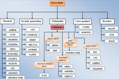
Force Field: Force field is the mathematical functions/parameters which are employed to describe the potential energy of the molecules and the atoms in context of molecular modeling. These force field functions and parameters are resultant of experimental and high-level quantum mechanical calculations. Basically, these parameters are designed according to a) ‘All-atom’, b) ‘United-Atom’ and c) ‘Coarse-grained’ force fields. All-atom force fields are used for all type of small atoms in the system together with hydrogen while United-Atom force fields are used for specific large atoms e.g. methyl molecule and other molecules. Similarly, the Coarse-gained force-field is frequently used in the long-term simulation of the proteins 11.
Types of Force Fields: The force fields can be broadly classified into five different categories depending on their usage in different systems starting from classical to modern modus operandi.
Starting from classical to second generation force fields, newer dimensions were added later on. For
e.g. AMBER is generally used for simulating DNA structure to find out the most suitable conformation
12
. Moreover, newly discovered force field named as ‘parmbsc1’ and SIRAH are very useful for atomistic simulation of almost DNA structure space
13, 14
. The polarizable force fields came up based on the different charges and theories.
FIG. 2: FORCE FIELD AND THEIR CLASSIFICATION ACCORDING TO DIFFERENT SYSTEMS REQUIREMENT
AMBER (Assisted Model Building and Energy Refinement), CVFF (Consistent Valence Force field), CHARMM (Chemistry at HARvard Molecular Mechanics) CHARMm (commercial version of CHRAMM), COSMOS-NMR (Computer Simulation of Molecular Structures-NMR),GROMOS (GROningen MOlecular Simulation package) OPLS (Optimized Potential for Liquid Simulations), OCFF/PI (Quantum Mechanical Consistent Force Field), UFF (Universal Force Field), CFF (Consistent Force field), COMPASS (Condensed-phase Optimized Molecular Potentials for Atomistic Simulation Studies), MMFF (Merck Molecular Force Field), MM2/3/4 (Molecular Mechanics 2/3/4), QVBMM (Quantized Valence Bonds′ Molecular Mechanics), TraPPE (An Acronym for Transferable Potentials for Phase Equilibria), X-pol (Explicit Polarization theory), DRF90 (Direct Reaction field), PIPF ( Polarizable Intermolecular Potential for fluids), VAMM (Virtual Atom Molecular Mechanics), MARTINI (same as name), SIBFA (Sum of Interactions Between Fragments Ab-initio Computed), AMOEBA (Atomic Multipole Optimized Energetic for Bimolecular Applications), ORIENT (same as name), CPE (Chemical Potential Equalization), PFF (Polarizable Force Field), ReaxFF (reactive force field), EVB (Empirical Valance bond) & RWFF (Reactive Water Force Field).
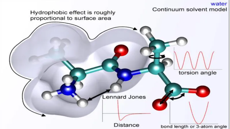
Force Field Function Calculation: The function of the force field can be calculated for bonded and non-bonded molecules and atoms. The precise decomposition of the terms depends on the force field and is defined as the term of the energy of bonded and non-bonded term
(1)
The component of bonded and non-bonded depends on the covalent and non-covalent bond interactions expressed by the following equations:
(2)
(3) In the presence of force field, the bond and angle term are usually modeled as harmonic oscillators
which prevent them from bond breaking. The Morse potential provides the more practical description for a covalent bond at higher stretching in which the potential energy is written as quadratic forms of internal energy as well as bonding energy modeled by the quantum harmonic oscillator. The non-bonded term includes many more interactions per atom which are computationally intensive. Generally, electrostatic and van der Waal interaction energies are calculated.
FIG. 3: DIFFERENT FORCES APPLIED TO A MOLECULE WITH CONTINUUM SOLVENT LIKE WATER
http://en.wikipedia.org/wiki/Force_field_%28chemistry%29#mediaviewer/File:MM_PE
Classical Mechanics in MD: MD provides solutions based on classical equations of the atoms and molecules based on the time evolution of the systems. MD is based on Newton’s second law of motion and for ith particle of the system can be given as
(4)
Where Fi is the applied force field on mass mi of particle i and ai is the acceleration of ith particle. The acceleration of the ith particle in the system can be determined if we know the applied force on particle and expressed as
(5)
Where viis the velocity of the ith particle and it is the second derivative of displacement of the particle with respect to time. Moreover, the acceleration of the particle can be represented as the derivative of the potential energy with respect to the position ri, of the ith particle in the system
(6)
The force can expressed as the gradient of the potential energy,
(7)
Combining the equation of 1 and 4
(8)
Where, V represents the potential energy of systems. This Newton’s equation of motion shows the relationship between the derivatives of potential energy to the change in the position of the ith particle as the function of the time in the system. Initially, allocation of velocities is generally identified from a random distribution and magnitudes provide the required temperature and corrected. Hence there is no overall momentum, i.e.
(9)
The velocities viare often chosen randomly from a Gaussian distribution or Maxwell-Boltzmann at a certain temperature which provides the probability that an atom i has a velocity vx in the x direction at
a temperature T.
(10)
(11)
Where N is the number of the atoms in the system
15, 16
.
Different integration algorithms are used to integrate the motion equations which capture the positions and movements of the particle and noted trajectory files. The trajectory file contains the description of particles positions, particles velocities and particles acceleration, which vary with respect to time. The average values of the particle behavior in the system are also noted the trajectory files. Hence integration algorithms help in the calculation of the positions, velocities of each atom and the state of the system
Integration Algorithms: In a bio-molecular system, the atomic positions (3N) of all atoms, is the function of potential energy. This potential energy function is complicated in nature and there is no analytical solution for the equations of motion, hence the motion equation has to be solved numerically. Many numerical algorithms have been developed for integrating the equations of motion. These algorithms are mainly Beeman’s algorithm, Verlet algorithm, Velocity Verlet, and Leap-frog algorithm. Before choosing integration algorithms, it is important that the user must consider the algorithm whether it is computationally efficient, conserve energy & momentum and allow a long time step for integration 17.
Verlet Algorithm: Most commonly used time integration algorithm in MD simulation and computer graphics is Verlet algorithm. Verlet integration is used to integrate Newton’s equation of motion and to generate the trajectories of the particle 18. In 1960s, this algorithm was used by Loup Verlet for MD for the first time. In 1907, Carl Stormer used to study the electrical particles motion in the magnetic field. Later in 1909, Cowell and Crommelin used to calculate the orbit of Halley’s Comet. The numerically stable Verlet integrator provides the time reversibility in physical system and prevention of the simplistic form on phase space 19.
Generally, integration algorithms presume the velocities (vi), positions (ri) and accelerations (ai) can be approximated by a Taylor series expansion.
Expanding the position of the ith particle having ri position at time t + ∆t and t - ∆t and bi as the third derivative of ri
(12)
(13)
O(∆t4
) is local error in position of Verlet integrator. Adding the expression (12) and (13)
(14)
Equate equation (14) by putting ai= Fi / mi
(15) The equation (12) and (13) constitute the basic form of the Verlet algorithm. As we are integrating Newton's equation, ai = Fi / mi x(t), the force is in turn a function of the positions ri(t:)
(16)
This version of Verlet algorithm has a problem, in directly generating the velocities. At the same time as they are not required for the time evolution, their information is sometimes necessary. In addition, they are necessary to calculate the kinetic energy K, whose assessment is essential to test the conservation of the total energy E=K+V. From this assessment, one can validate that a MD simulation is taking place correctly. One could compute the velocities from ith positions by using
(17)
Still, the fault linked to this expression is the order of ∆t2 rather than ∆42. To come out this complexity, some alternatives have been developed and described in next section 18.
algorithm use an approximation for derivative, one should consider the velocity vi at the midpoint between times (t) and (t + ∆t) and express as:
(18)
The equation (18) can be solved in term of ri (t +
∆t) and yield
(19)
In the same way, the velocity can also define in the midpoint of (t - ∆t) and (t) as given below
(20)
The acceleration ai at time (t) can be defined using appropriate formula for the derivative,
(21)
By means of Newton’s equation for the acceleration ai(t)= Fi (t) / mi and putting the value to equation (21) yields
(22)
Equation (22) can be solved for vi (t + ∆t / 2),
(23)
Equations (16) and (20) comprise the equations of
Verlet leapfrog algorithm. It has mainly two advantages which are not present in the original Verlet algorithm (11). (I) in original Verlet algorithm the loss of accuracy due to round-off error is resolved. (II) The original Verlet algorithm does not comprise of the explicit velocities which are included in Verlet leapfrog algorithm. The algorithm still has associated problems like it is still not self-starting. This problem can be solved as in the original Verlet method by implementing one step of the Euler method first and then switching to the Leapfrog algorithm for subsequent steps 20 - 21. Velocity Verlet: The Velocity Verlet was developed to overcome the associated problem related to
Verlet algorithm. This algorithm is analogous to
leapfrog method apart from that the velocity and position are calculated at the same time interval while the leapfrog method does not perform same. The Velocity Verlet’s different form can be obtained from the original Verlet algorithms in which positions ri, velocities vi and acceleration ai at the time (t + ∆t).
(24)
(25)
(26)
(27)
Note that long-term outcome of Velocity Verlet and Leapfrog is one order better than the semi-implicit Euler method. These algorithms are almost identical up to half velocity time step. The Velocity Verlet differs only while considering midpoint velocity as the final velocity in semi-implicit Euler method. The method has the error of order two which is similar to the midpoint method 22.
Beeman’s Algorithm: Beeman’s Algorithm is the method that provides the numerical integration of ordinary differential equation of order two, more distinctively Newton’s equation of motion. The algorithm is designed in such a way that allows high numbers of particles in MD simulation. It uses a direct or explicit and an implicit variant of the method. In 1973 the Schofield published the direct variant which is commonly known as Beeman’s method 23. This is alternative of the Verlet integration method and creates identical position but uses a different formula for the velocity calculation.
Later in 1976, Beeman published a class of implicit (predictor-corrector) multi-step methods in which the Beeman’s methods itself is a variant of the third order method in this class 24. The full predictor-corrector computes the position riof particle at time
(t + ∆t) form data at times t and (t - ∆t)
(29)
(30)
The equation (30) can be represented as an alternative by updating the velocity using second-order Admas-Moulton Method
(31)
Ensembles: An ensemble is a large group of microscopically described states of a system with certain constant macroscopic properties. In MD simulations it is used to achieve quantitative outcome under various thermodynamic conditions for realistic models which are parameterized to study a specific molecular or atomic system with a certain degree of realism. It consists of transferable parameters for molecular sub-units usually at the atomistic level. Generally, Microcanonical ensemble (NVE), Isothermal-isobaric ensemble (NPT) Canonical ensemble (NVT), and some other gene-ralized ensembles are used in MD simulation 25. Microcanonical Ensemble (NVE): A system (solid, liquid or gas) is completely isolated from changes in volume (V) having the constant number of particles (N) and Energy (E). An adiabatic process with no heat exchange is similar the NVE ensemble. In the ensemble, the exchange of kinetic and potential energy with total energy may be seen. A system of particles N with X coordinate and velocities V having potential energy U, the following pair may be expressed in terms of first order differential equation of Newton’s notation as
(32) (33)
Where U(X) is the potential energy function of system. The force F acting on each particle of the system can be calculated as the negative gradient of
U(X) 26, 27.
Canonical Ensemble (NVT): Canonical ensemble has volume (V), particles (N) with a contact of heat bath with constant temperature (T). Hence, it is also referred as Constant Temperature Molecular Dynamics (CTMD). The energy of exothermic and endothermic processes is exchanged with a thermo-
stat (discussed in next section) in canonical ensemble 26, 27.
Isothermal-isobaric Ensemble (NPT): Isothermal -isobaric ensemble is a statistical mechanical ensemble having (N) particle with constant temperature (T) and pressure (P).The thermostats and barostat correspond most closely to laboratory conditions with a flask open to ambient temperature and pressure. NPT ensemble plays an important role in chemistry as chemical reactions are regularly carried out under constant pressure condition. For simulation of biological membranes, isotropic pressure control is not appropriate. Hence in the simulation of lipid bilayers, pressure control under constant membrane area (NPAT) and the constant surface tension "gamma" (NPγT) ensemble is generally recommended 27.
Generalized Ensemble: The best method of a generalized ensemble is replica exchange and was created to handle the slow dynamics of the disordered spin system. It is also known as parallel tempering. To overcome, the multiple-minima problem the replica exchange MD formulation is used and obtained by exchanging the temperature of non-interacting replicas of the system running at several temperatures.
TABLE 1: LIST OF DIFFERENT THERMOSTATS AND THEIR BRIEF DESCRIPTION ARE USED IN MD SIMULATIONS
Thermostat Description Canonical? Stochastic? Advantages Disadvantages
Velocity rescaling
Rescaling of the velocity performs at every time steps by fixing kinetic energy (KE) to match the Temperature of MD.
The desired temperature obtained by multiplying each atomic velocity by factor.
No No Straight-forward to code.
Good for use in initialization step.
Results do not correspond to any ensemble; while in practice the amount they deviate from canonical is quite small and not permit the correct temperature fluctuation. Not advised to employ in production
MD runs. Since they do not strictly conform to the canonical ensemble, but fine to use during equilibration. Unwanted or localized correlation
motion not removed. Berendsen Another popular velocity rescaling
method.
The scaling is obtained as
where, r is ‘rise time’ of thermostat. It explain power of the coupling of the to a hypothetical heat bath.
No No Straight-forward to implement.
Method is robust
Results do not correspond to any ensemble, while in practice; the amount they deviate from canonical is quite small.
Not advised for use in production MD runs since they do not strictly conform to the canonical ensemble, but fine to use during equilibration. Localized or unwanted correlation
motion not removed. Nose-Hoover
chain
Based on extended Lagrangian formalism.
Based on elegant formalism proposed by Nosé (1984), in which micro-canonical dynamics on this extended system is revealed to give canonical properties.
Deterministic and time reversible. Hamiltonian is given as
Logarithmic term required for
proper time scaling: canonical ensemble.
Effective mass Q associated with S, if Q too small: system not canonical or Q too large: temperature control inefficient.
Micro-canonical dynamics on extended system give canonical properties
Yes No Easy to implement and use. This implements as chain and each link apply the thermo stating to the previous thermo-stat variable. Deterministic and time
reversible.
Increasing Q lengthens decay time in response to instantaneous temperature jump.
Extended system not sure to be ergodic.
Becoming trapped in subspace– thus dangerous as a thermostat
Langevin Consider the motion of large particles through a continuum of smaller particles
Viscous drag force proportional to velocity γ Pi
Smaller particles give random pushes to large particle. Fluctuation –dissipation relation.
Yes Yes The behavior of dynamics samples from canonical ensemble is properly thermal for temperature T. Shown as ergodic. Local heat bath
coupled on each particle. This process removes heat trapped in localized modes. Accord to use a larger
time step compared to non-stochastic thermostats.
Momentum transfer is destroyed cannot compute diffusion coefficients.
Difficult to implement drag for non-spherical particles.
Andersen Possibly the easier thermostat which having correctly sample of the NVT ensemble.
Couple a system to a heat bath to impose desired temperature. Equations of motion are
Hamiltonian with stochastic collision term.
Strength of coupling specified by v, the stochastic collision frequency. When particle has collision, new
velocity is sampled from N (O,√T)
Yes Yes Samples are from canonical ensemble. While a Langevin
trajectory, over time, drifts away from the ‘perfect’ (energy conserving) path due to noise and drag, the Andersen trajectory is perfectly energy conserving.
The mixing of Newtonian dynamics with stochastic collisions turns the MD simulation into a Markov process.
Limitation of MD Simulation: There are mainly three limitations are observed when MD simulation was carried out. The limitations are force field dependency, Neglect of Electronic motion and critical frequencies and how they affect the simulation results described below.
Force Field Dependency: The various force fields are designed for the different bio molecules systems like for protein GROMOS and for DNA it is AMBER. The MD simulation can only provide good results if the force field is applied in accordance with the relevant bio molecules otherwise the results will get affected.
Neglect of Electronic Motion: The classical MD follows only the particle nuclear motion while the electronic motion and quantum effects are ignored. Hence, the classical MD is unsuitable for chemical bonding of metal ions and chemical reactions. Quantum dynamics approaches are used for this purpose which is very typical and complex to design as such programs also need high computational power and efficiency.
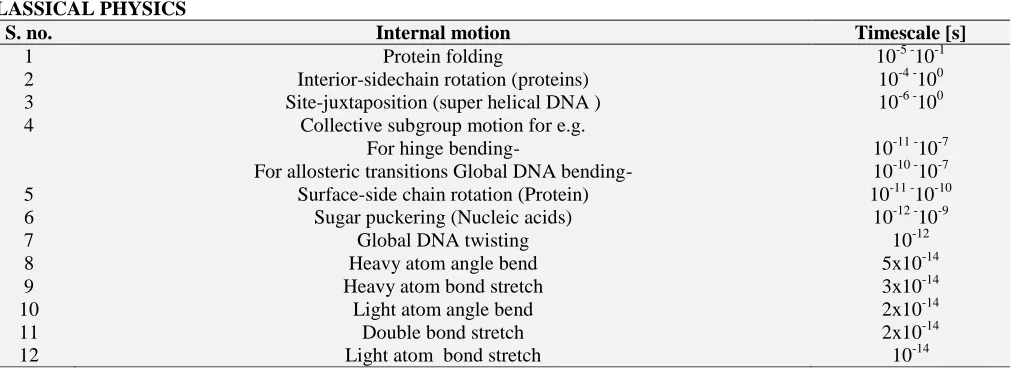
Critical frequencies: There is a considerable amount of evidence found when we apply the forces and thermostats in the bio-molecular system. One of the most important evidence is the critical frequency of the bonded atom. In general, the critical frequency is the spontaneous oscillation of connected atoms of the system. The classical MD is inappropriate to calculate such vibration at low temperatures where the quantum effects are more suitable. Generally, the quantum effect calculates on the basis ofhʋ = kBT .Wheneverhʋ > kBT, then we should be concerned about the quantum effect. There is some ratio of high-frequency vibrations at T=300K listed in Table 2. The hʋ / kBT ratio >1 shows such high frequency vibrational modes are not handled by the classical physics. Moreover, the Newtonian physics calculation shows that energy is equally distributed among the vibrational modes if
hʋ / kBT ratio~1. Hence, picoseconds range and longer timeframes time scales are reasonably treated by the classical physics. The Table 3 showing the broad spectrum of characteristic time scales in bio-molecules which is generally required to simulates a bio molecules.
TABLE 2: THE CALCULATED FREQUENCY, WAVE NUMBER AND THEIR RATIO ARE GENERATED BY DIFFERENT VIBRATIONAL MODE
Vibrational mode Frequency ʋ[s-1] Wave number (1/λ) [cm-1] Ratio hʋ / kBT
O-C-O bend 2.1 x10¹³ 700 3
C-N stretch (amines) 3.8 x10¹³ 1250 6
C=O stretch(carbonyl) 5.1 x10¹³ 1700 8
O-C-O asymmetric stretch 7.2 x10¹³ 2400 12
C-H stretch 9.0 x10¹³ 3000 14
O-H stretch 1.1 x10¹⁴ 3600 17
TABLE 3: DIFFERENT TYPES OF BIMOLECULAR MOTION AND THEIR TIME SCALE ARE OBSERVED IN CLASSICAL PHYSICS
S. no. Internal motion Timescale [s]
1 Protein folding 10-5 -10-1
2 Interior-sidechain rotation (proteins) 10-4 -100
3 Site-juxtaposition (super helical DNA ) 10-6 -100
4 Collective subgroup motion for e.g.
For hinge bending-
For allosteric transitions Global DNA bending-
10-11 -10-7 10-10 -10-7
5 Surface-side chain rotation (Protein) 10-11 -10-10
6 Sugar puckering (Nucleic acids) 10-12 -10-9
7 Global DNA twisting 10-12
8 Heavy atom angle bend 5x10-14
9 Heavy atom bond stretch 3x10-14
10 Light atom angle bend 2x10-14
11 Double bond stretch 2x10-14
12 Light atom bond stretch 10-14
Other Bimolecular Simulation Methods: This section explains about other simulation methods
[image:10.612.49.564.416.502.2] [image:10.612.58.564.524.708.2]Monte Carlo Method: The Monte Carlo method is a stochastic simulation technique which approximates the probabilities of large numbers of microstates or configurations of equilibrated systems generated by random sampling using Monte Carlo integration and statistical tests. In the 1930s, first time Enrico Femi used Monte Carlo method to study the neutron diffusion and that experiment was not published anywhere. Later on, in the late 1940s, Stanislaw Ulam discovered modern version of Monte Carlo method while working on nuclear weapons project at the Los Alamos National Laboratory. The name Monte Carlo comes from the similar technique playing and recording results in a real gambling casino. The method is frequently utilized in the problems of physics and mathematics and is most useful when it is difficult to achieve a closed-form expression, or infeasible to apply a deterministic algorithm. Generally, the Monte Carlo methods are used in three diverse classes of problems which are optimization, numerical integration and probability distribution
29
.
Brownian Dynamics: Brownian Dynamics is an efficient mesoscopic simulation method for bio-molecules in which explicit solvent bio-molecules are reinstated as an alternative of stochastic forces. This approach uses viscous continuum/more sluggish motion colloides or polymer as a solvent, which allows one to simulate in long time scale. The stochastic force applied to the macromolecules which initiate random collusion in the solvent molecules in this way Brownian motion in the system initiate and changes in different time scale. Further in a schismatic differential equation integrates forward in time and generates the trajectory of molecules. Brownian dynamics includes the simulation of particles that undergo Brownian motion and follows the simplified version of Langevin dynamics (LD) 30.
Let us consider the particles having a small mass and it is common to neglect the inertia of these particles. By applying the second law of Newton’s for particles i, Fitot = mi ai, Here inertia was ignored since the total force is always approximately zero. The total force on a particle consists of drag force
Fid, Brownian force FiB, and all non-hydrodynamic forces Finh. The Fid due to particle motion through viscous solvent, FiB generates due to random collisions of the solvent with the particle while Finh includes any external body forces any spring forces and any excluded volume interactions.
Fitot = FiB + Fid + Finh ~ 0 (34)
In a crawling flow and neglecting hydrodynamic interactions, the drag force is taken as Stokes drag on a sphere and it can be defined as
(35) Where ∑ is the dog coefficient and u∞ (ri) is the unperturbed velocity of the solvent evaluated at the position of the particle. The motion governing differential equation of the particle becomes as
(36)
and is known as Langevin equation, where {ri} is the set of all partials positions on which non-hydrodynamic force depends. This equation is also called stochastic differential equation because the Brownian force is taken from random distribution 31.
Different Algorithms and Software: Various algorithms and software were devolved to perform the bimolecular simulations are listed in Table 4, describe their name, functions, dependency on GUP and web link of availability.
TABLE 4: LIST OF FREELY AND COMMERCIALLY AVAILABLE SOFTWARE FOR BIMOLECULAR SIMULATION WHICH USES CLASSICAL MECHANICS AND QUANTUM MECHANICS PROPERTIES
S. no. Name Description GPU License Web-references
1 Abalone Provides the platform for molecular modeling and MD simulation of bio-molecules especially for biopolymers.
Use AMBER and OPLS force field.
Yes Free http://www.biomolecular-modeling.com/Abalone/index.htm
l 2 ACEMD Production-class bio-molecular dynamics engine uses
CHARMM and AMBER force field.
Running on NVDIA GPUs (Graphics processing unit) and heavily optimized with CUIDA. Specially designed for GPU and have ability to
Yes Basic version free Commercial version also available
http://www.acellera.com/products
[image:11.612.50.563.648.753.2]accomplish supercomputing performance of 40ns/day for all-atom protein system with over 23000 atoms. 3 ADUN Includes tools for the calculation and analysis of
several dynamical properties of macromolecules. User specified CHARMM; AMBER forced field implemented using Force field markup language (FFML).
Empirical valence Bond (EVB) used for the calculation QM and MM.
Yes Free http://adun.imim.es/
4 AMBER Assisted Model Building with Energy Refinement (AMBER) is a family of force field used for MD of Bio-molecules and also known as software package. Tools use all AMBER force field only.
Yes Paid http://ambermd.org/
5 Ascalaph Designer
A general purpose tool for molecule design and MD simulation.
Provides the graphical environment to molecular molding and MD program like ORCA, NWChem, CP2K, Firefly, MDynaMix and GAMESS.
Yes Free (GNU GPL) & Commercial
http://www.biomolecular-modeling.com/Products.html
6 CHARMM Chemistry at HARvard Macromolecular Mechanics (CHARMM) is a flexible and widely used MD Simulation program for bio-molecules.
Commercially available in the Discovery Studio for MD.
Yes Paid http://www.charmm.org/
7 COSMOS
Provides MM and MD simulation through Quantum chemistry calculation of chemical shifts and atomic charges with an accuracy that compares to ab initio calculations.
No
Free (Without GUI)
http://www.cosmos-software.de/ce_intro.html
8 CP2K CP2K can execute atomistic, molecular simulations of solid state, liquid and biological systems.
Yes Free for GNU http://cp2k.org/ 9 Culgi Provides atomistic and mesoscale MD Simulation. No Paid https://culgi.com/ 10 Desmond A tool developed at D.E. Shaw Research Foundation
to perform high speed MD simulation of Bio-molecules and commercially available in Schrodinger.
The CHARMM (22,27,32,36), AMBER (94,96,99,03) and OPLS (2001, 2005) as well as other in house developed force field variant is suppurated by Desmond.
Yes Free and Commercial
http://www.deshawresearch.com or
http://www.schrodinger.com/Des mond
11 Discovery Studio
A well known software package provides major solution of Structural Biology focused on the optimization of drug discovery process.
Provides Small molecule simulation as well as large bio molecules MD simulation using CHARMM, MMFF, MOL3, QUANTUMM and CFF.
No Commercial and trail is available
http://accelrys.com/
12 GROMACS GROningen MAchine for Chemical Simulations (GROMCS) is a MD simulation packages for protein, lipids and Nucleic acid and developed at University of Groningen, Netherlands.
Available for CPU and Normal system user and provides all version GROMOES, AMBER and CHARMM fold field parameter.
Most preferable worldwide used software for MD Simulation.
Yes Free http://www.gromacs.org/
13 HOOMD-blue
Uses various pair potentials i.e. dissipative particle dynamics, Brownian dynamics, rigid body constraints, energy minimization, etc. General-purpose simulation tool highly
optimized for GPUs.
Yes Free http://codeblue.umich.edu/hoomd -blue/index.html
14 LAMMPS Large-scale Atomic/Molecular Massively Parallel Simulator (LAMMPS) is MD simulation program developed by Sandia National laboratories.
Yes Free http://lammps.sandia.gov/
15 Macro- Model
A classical mechanics based program used for molecular modeling and also carry out simulations. Use stohastics dynamics and mixed Mante Carlo
algorithms to perform MD at finite temperature.
No Paid http://www.schrodinger.com/Mac roModel
16 MAPS Materials Processes and Simulations (MAPS) provide the visualization and analysis with multiple simulation engines.
Yes Closed source/Trial
available
http://www.scienomics.com/prod
ucts/molecular-modeling-platform/ 17 MedeA Combines computational programs like Vienna.
A-Initio Simulation Package (VASP) LAMMPS, GIBBS for material MD simulations.
No Paid/Trial available
18 Q Designed for special kinds of free energy calculation which are free energy Perturbation (FEP) simulation, Empirical valence bond (EVB) calculates the reaction free energy and linear interaction energy used for protein ligand binding affinities. The available force field are GROMOS87/96,
AMBER95, OPLS and CHARMM22
No Free for non-commercial use
http://xray.bmc.uu.se/~aqwww/q/
19 RedMD Provides the MD simulations in a microcanonical ensemble, with Berendsen and Langevin thermostats, and with Brownian dynamic.
No Free on GNU License
https://bionano.cent.uw.edu.pl/sof tware/redmd 20 SCIGRESS Best use for MM calculations on the organic and
inorganic molecules containing all elements of the periodic table using verity of force field.
No Paid http://www.fqs.pl/Chemistry_Mat erials_Life_Science/products/scig
ress 21 TeraChem First computational chemistry software enabling
quantum chemistry and first principles dynamics for molecular materials and biological molecules. Designed algorithms exploit massive Parallelism of
CUDA-enabled NVIDIA GPUs.
Yes Paid http://petachem.com/
22 TINKER Provides the molecular mechanics (MM) and MD for bio molecules with some special features for the biopolymer.
No Free http://dasher.wustl.edu/tinker/
23 Termolo-X Generally used for the numerical simulation of interactions between atoms and molecules.
No Paid http://www.tremolo-x.com/overview.html 24 NAMD NAosecale Molecular Dynamic Program (NAMD)
for MD simulation developed in the Charm++ parallel programming model.
The parallel molecular dynamic code allowing the interactive simulation in the platform of VMD.
Yes Free for academics http://www.ks.uiuc.edu/Research/ namd/
25 YASARA Yet Another Scientific Artificial Reality Application (YASARA) is a molecular visualization, modeling and MD simulation tool.
Powered by Portable Language (PVL)
No Paid http://yasara.org/
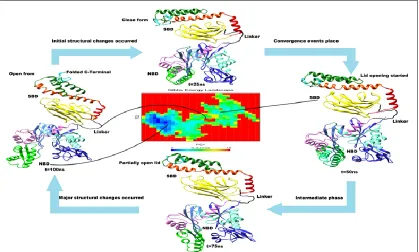
Application of MD Simulation: MD simulation is used to explore the complex biochemical processes such as: (I) study of protein folding and mutation analysis, (II) exploration of protein motion as essential for the identification of the protein function, (III) Study of DNA, RNA folding and opening process, (IV) Elucidation of bimolecular complex stability (Protein-protein, Protein-DNA, Protein-RNA, Protein-ligand), (VI) treat collision cascades in the heat spike regime and (VII) Explore the role of temperature in various thermodynamics studies. Indeed various works have been performed to explain these applications of molecular dynamics simulation some of them are explain in subsection. Study of Protein Folding and Mutation Analysis: Recently, Gupta et al., 2015 explored the protein folding and interdomain communication event of heat shock protein 70 (HSP70) through MD simulation. The study explains how the confirmation of HSP70 proteins changes from open state to close state. The results also provide a mechanistic representation of the communication between nucleotide binding domain (NBD) and substrate binding domain SBD. This identifies the different role of subdomains in conformational change mechanism, which leads the chaperone cycle of cHSP70 32. Fig. 4 explains how the HSP70 obtained
stress. PIs produce by the plant during pests attack and function as pseudosubstrates for the digestive protein of pests. As a result inhibition of pro-teolysis process in pests occurs, this leads towards amino acid-based mortality. Further, the structural interaction analysis of serine proteinase of
[image:14.612.98.517.147.399.2]Heterodera glycines (SPHG) with Vigna mungo proteinase inhibitor (VMPI) though Protein-protein docking followed by MD simulation. Study mimics the protein-protein interactions affinity through MD simulation 34.
FIG. 4: THE STRUCTURAL AND FOLDING EVOLUTION OF CAMEL HSP70 PROTEIN CALCULATED DURING 100 NS OF MD SIMULATION.
The averaged structure of 25 ns interval is depicting their different folding sate. Gibbs free energy landscape stand for the frequency of subunit folding identified via Principal Component I and II Analysis (PCA). The minimum Gibbs free energy (blue color spot) shows minimum folding rates in domains while the intermediate and higher energy (green and yellow spots) shows intermediate and higher folding rate in subunit of HSP70 whole simulation is performed by Gupta et al., 2015(adapted with permission from 30)
The post-transcriptional gene regulation depends not only on the mRNAs sequence but also on their folding into complex secondary structures and chemical modifications of RNA bases. These features of RNA are highly dynamic and independent and having their direct control in the transcriptome, which leads changes in several functions of the cell 35. Hence, it is important to analyze the coupling of RNA structures and its modifications and RNA–protein interactions at different steps of the gene expression process 36. Recently, Chhaya et al., 2017 performed the MD simulation using AMBER tool to mimic various isoforms of preE-let7 in complex with LIN28 protein which inhibits the biogenesis miRNAs of let-7 family. Further, they also identified structural features and key specificity determining residues (SDR) crucial for the inhibitory role of LIN28 37.
Similarly, exploration of interaction analysis between protein-DNA complexes through simulation is also helpful to elucidate DNA-binding specificities a gene expression process. For example to analyze stimulus-specific responses of conserved WRKY DNA-binding domain (DBD) completely recognize the ‘TTGACY’ W-box consensus. We speculated that the W-box consensus might be more degenerate and yet undetected differences in the W-box consensus of WRKYs of different evolutionary descent exist. Simulation analysis was performed to explore differences in DNA-binding specificities 38.
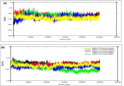
of proteins responsible for various phenotypic and genotypic changes. Gupta et al., 2015 explained the protein-ligand complex stability in context to identify the suitable lead compounds for the
[image:15.612.95.524.118.414.2]treatment of malaria 39. Fig. 5 indicating interaction energy and folding rate plot of top five complexes during 25 ns of MD simulation.
FIG. 5:THE INTERACTION ENERGY AND FOLDING RATE OF PROTEIN-LIGAND COMPLEX STRUCTURES OF STUDY PERFORMED BY GUPTA et al., 2015
(a) The LJ-SR protein–ligand interaction energy graph and (b) radius of gyration (Rg) plot of each complex during 25 ns simulation (adapted with permission from 37)
Study of DNA, RNA Folding, and Opening Process: DNA and RNA are involved in the processing of genetic information at different levels of the cell. To address, how DNA, RNA molecules performed their functions, it is required to understand the structure and dynamics of DNA/RNA at the atomistic level. This can be feasible to analyses them through MD simulation with experiment. Different types of simulations are performed to identify the details DNA, RNA molecules and their interactions with systems solvent, ions and peptides/proteins. Further, it describes structural and dynamical insights of these biomolecules and explains its transition from one state to another state 44 - 48.
Recently, Dens et al., reviewed the multiscale simulation of DNA and discussing most recent theoretical methods used to study DNA and classified these methods into four groups as per their level of resolution (Fig. 6): (i) electronic, (II)
atomistic, (III), coarse-grained, and (IV) mesoscopic. It is not true that if we are moving words resolution space that means moving also in methodological space. Fig. 6 a, 6b, 6c and 6d highlighting different methods based DNA/RNA simulation: (a) the joint QM/MM work from the Magistrato’s group, explaining the atomistic and energetic variations of human Flap endo-nucleases (FENs) with DNA and RNA complex using mixed quantum-classical (QM/MM) meta-dynamics and umbrella sampling free energy calculations 49. (b) Explains how DNA Holliday-junction simulated with the new force parmBSC1
13
also performed using MD simulation and we recommend researcher to read specific articles to
execute and understand deeper MD simulation analysis.
FIG. 6: SCHEME ILLUSTRATING THE INTRINSIC MULTISCALE NATURE OF DNA
The models and applications are sorted in this scheme according to five dimensions i.e. time scale, size scale, methodological space, models and resolution (adapted with the permission from, 46). They have highlighted four applications of MD simulation (a) the combined QM/MM work from the Magistrato’s group, were a protein-DNA complex with a DNA lesion is studied in detail 18. (b) Holliday-junction simulated with the new parmBSC1 refined force-field for DNA simulations, adapted from 13. (c) LacI-DNA dynamics by multiscale simulations using the SIRAH force-field from Pantano’s group 14. (d) The model from Schlick and coworkers was used to study the chromatin fiber dynamics. Chromatin fibers in the canonical and hairpin-like conformations are depicted (adapted with permission from 50.
CONCLUSION: In this review, a brief outline has been given emphasizing the key elements which are essential to carry out a molecular dynamics simulation, with special emphasis on bio-molecular systems. We have discussed different steps involved in the MD simulation with the necessity of each of them. Also, MD applications and MD limitations were described with assumptions of classical mechanics, molecular mechanics, force fields and integration algorithms.
Moreover, we have briefly described the concept of ensembles and thermostats and its practical use in certain simulation. Bio-molecular simulation methods and various MD simulation programs and software tools available as open source and commercial domain were explained. Finally, different applications of MD simulation with recent work is discussed, indicates their role to understand bio-molecules functions.
ACKNOWLEDGEMENT: Authors would like to
thank Indian Institute of Information Technology-Allahabad, for providing all facilities to complete this review paper.
CONFLICT OF INTEREST: Authors affirm that they do not have any conflict of interest.
REFERENCES:
1. Alder BJ and Wainwright T: Phase transition for a hard sphere system. The Journal of chemical physics. 1957; 27 (5): 1208-9.
2. Alder BJ and Wainwright TE: Studies in molecular dynamics. I. General method. The Journal of Chemical Physics. 1959; 31(2): 459-66.
3. Rahman A: Correlations in the motion of atoms in liquid argon. Physical Review. 1964; 136(2A): A405.
4. Karplus M and Petsko GA: Molecular dynamics simulations in biology. Nature. 1990; 347(6294): 631-9. 5. Karplus M and McCammon JA: Molecular dynamics
simulations of biomolecules. Nature Structural and Molecular Biology. 2002; 9(9): 646-52.
6. Borhani DW and Shaw DE: The future of molecular dynamics simulations in drug discovery. Journal of Computer-aided Molecular Design. 2012; 26(1): 15-26. 7. Kuehn K: Newton’s Laws of Motion. In a student's guide
through the great physics texts, Springer New York, 2015: 261-264.
8. Berendsen HJ, Postma JP, van Gunsteren WF and Hermans J: Interaction models for water in relation to protein hydration. In intermolecular forces, Springer Netherlands, 1981: 331-342.
10. Ponder JW and Case DA: Force fields for protein simulations. Advances in protein chemistry. 2003; 66:27-85.
11. Leckband D and Israelachvili J: Intermolecular forces in biology. Quarterly reviews of biophysics. 2001; 34(2): 105-267.
12. Ivani I, Dans PD, Noy A, Pérez A, Faustino I, Hospital A, Walther J, Andrio P, Goñi R, Balaceanu A and Portella G: Parmbsc1: a refined force-field for DNA simulations. Nature methods. 2016; 13(1): 55.
13. Machado MR and Pantano S: Exploring LacI-DNA dynamics by multiscale simulations using the SIRAH force field. Journal of chemical theory and computation. 2015; 11(10): 5012-23.
14. Goldstein H: Classical mechanics. Pearson Education India; 2011.
15. Håkan HW and Ågren H: Quantum mechanics/classical mechanics modeling of biological systems. In Multiscale Modeling and Simulation in Science, Springer, Berlin, Heidelberg, 2009: 291-294.
16. Hentschke R: Integrating the equations of motion. In Classical Mechanics, Springer International Publishing, 2017: 123-153.
17. Verlet L: Computer" experiments" on classical fluids. I. Thermodynamical properties of Lennard-Jones molecules. Physical review. 1967; 159(1): 98.
18. Koobus B and Farhat C: Second-order time-accurate and geometrically conservative implicit schemes for flow computations on unstructured dynamic meshes. Computer Methods in Applied Mechanics and Engineering. 1999; 170(1-2): 103-29.
19. Cuendet MA and van Gunsteren WF: On the calculation of velocity-dependent properties in molecular dynamics simulations using the leapfrog integration algorithm. The Journal of chemical physics. 2007; 127(18): 184102. 20. Mikkola S and Aarseth S: A time-transformed leapfrog
scheme. Celestial Mechanics and Dynamical Astronomy. 2002; 84(4): 343-54.
21. Swope WC, Andersen HC, Berens PH and Wilson KR: A computer simulation method for the calculation of equilibrium constants for the formation of physical clusters of molecules: Application to small water clusters. The Journal of Chemical Physics. 1982; 76(1): 637-49. 22. Schofield P: Computer simulation studies of the liquid
state. Computer Physics Communications 1973; 5(1): 17-23.
23. Beeman D: Some multistep methods for use in molecular dynamics calculations. Journal of computational Physics. 1976; 20(2): 130-9.
24. Allen MP: Algorithms for Brownian dynamics. Molecular Physics. 1982; 47(3): 599-601.
25. Okamoto Y: Generalized-ensemble algorithms: enhanced sampling techniques for Monte Carlo and molecular dynamics simulations. Journal of Molecular Graphics and Modelling. 2004; 22(5): 425-39.
26. Nguyen TD, Phillips CL, Anderson JA and Glotzer SC: Rigid body constraints realized in massively-parallel molecular dynamics on graphics processing units. Computer Physics Communications 2011; 182(11): 2307-13.
27. Wereszczynski J and McCammon JA: Statistical mechanics and molecular dynamics in evaluating thermodynamic properties of biomolecular recognition. Quarterly reviews of biophysics 2012; 45(1):1-25. 28. Johnson A, Johnson T, Khan A. Thermostats in Molecular
Dynamics Simulations. University of Massachusetts Amherst 2012; 6: 1-29.
29. Rubinstein RY and Kroese DP: Simulation and the Monte Carlo method. John Wiley & Sons; 2016.
30. Doyle PS and Underhill PT: Brownian dynamics simulations of polymers and soft matter. Handbook of materials modeling. 2005: 2619-30.
31. Northrup SH, Allison SA and McCammon JA: Brownian dynamics simulation of diffusion‐influenced bimolecular reactions. The Journal of chemical physics. 1984; 80(4): 1517-24.
32. Gupta S, Rao AR, Varadwaj PK, De S and Mohapatra T: Extrapolation of inter domain communications and substrate binding cavity of camel HSP70 1A: a molecular modeling and dynamics simulation study. PloS one. 2015; 10(8): e0136630.
33. Maganhi SH, Jensen P, Caracelli I, Schpector JZ, Fröhling S and Friedman R: Palbociclib can overcome mutations in cyclin dependent kinase 6 that break hydrogen bonds between the drug and the protein: Supplementary Information.
34. Prasad CS, Gupta S, Gaponenko A and Tiwari M: Molecular dynamic and docking interaction study of Heterodera glycines serine proteinase with Vigna mungo proteinase inhibitor. Applied biochemistry and bio-technology. 2013; 170(8): 1996-2008.
35. Lewis CJ, Pan T and Kalsotra A: RNA modifications and structures cooperate to guide RNA-protein interactions. Nature Reviews Molecular Cell Biology. 2017; 18(3): 202-10.
36. Ellis JJ, Broom M and Jones S: Protein-RNA interactions: structural analysis and functional classes. Proteins: Structure, Function and Bioinformatics. 2007; 66(4): 903-11.
37. Sharma C and Mohanty D: Molecular dynamics simulations for deciphering the structural basis of recognition of Pre-let-7 miRNAs by LIN28. Biochemistry. 2017; 56(5): 723-35.
38. Brand LH, Fischer NM, Harter K, Kohlbacher O and Wanke D: Elucidating the evolutionary conserved DNA-binding specificities of WRKY transcription factors by molecular dynamics and in vitro binding assays. Nucleic acids research. 2013; 41(21): 9764-78.
39. Gupta S, Jadaun A, Kumar H, Raj U, Varadwaj PK and Rao AR: Exploration of new drug-like inhibitors for serine/threonine protein phosphatase 5 of Plasmodium
falciparum: a docking and simulation study. Journal of
Biomolecular Structure and Dynamics 2015; 33(11): 2421-41.
40. Kumar H, Raj U, Srivastava S, Gupta S and Varadwaj PK: Identification of dual natural inhibitors for chronic myeloid leukemia by virtual screening, molecular dynamics simulation and ADMET analysis. Inter-disciplinary Sciences: Computational Life Sciences. 2016; 8(3): 241-52.
41. Raj U, Kumar H, Gupta S and Varadwaj PK: Exploring dual inhibitors for STAT1 and STAT5 receptors utilizing virtual screening and dynamics simulation validation. Journal of Biomolecular Structure and Dynamics. 2016; 34(10): 2115-29.
42. Raj U, Kumar H, Gupta S and Varadwaj PK: el DOT1L receptor natural inhibitors involved in mixed lineage leukemia: a virtual screening, molecular docking and dynamics simulation study. Asian Pac J Cancer Prev. 2015; 16(9): 3817-25.
44. McDowell SE, Špačková N, Šponer J and Walter NG: Molecular dynamics simulations of RNA: an in silico single molecule approach. Biopolymers. 2007; 85(2): 169-84.
45. Gupta S, Kumari M, Kumar H and Varadwaj PK: Genome-wide analysis of miRNAs and Tasi-RNAs in Zea mays in response to phosphate deficiency. Functional & integrative genomics. 2017; 17(2-3): 335-51.
46. Pérez A, Luque FJ and Orozco M: Frontiers in molecular dynamics simulations of DNA. Accounts of chemical research. 2011; 45(2): 196-205.
47. Dans PD, Walther J, Gómez H and Orozco M: Multiscale simulation of DNA. Current opinion in structural biology. 2016; 37: 29-45.
48. Czapla-Masztafiak J, Nogueira JJ, Lipiec E, Kwiatek WM, Wood BR, Deacon GB, Kayser Y, Fernandes DL, Pavliuk MV, Szlachetko J and González L: Direct determination of metal complexes’ interaction with DNA by atomic Telemetry and multiscale molecular dynamics. The Journal of Physical Chemistry Letters. 2017; 8(4): 805-11. 49. Sgrignani J and Magistrato A: QM/MM MD simulations
on the enzymatic pathway of the human flap endonuclease (hFEN1) elucidating common cleavage pathways to RNase H enzymes. Acs Catalysis. 2015; 5(6): 3864-75.
50. Collepardo-Guevara R and Schlick T: Chromatin fiber polymorphism triggered by variations of DNA linker lengths. Proceedings of the National Academy of Sciences. 2014; 111(22): 8061-6.
All © 2013 are reserved by International Journal of Pharmaceutical Sciences and Research. This Journal licensed under a Creative Commons Attribution-NonCommercial-ShareAlike 3.0 Unported License.
This article can be downloaded to ANDROID OS based mobile. Scan QR Code using Code/Bar Scanner from your mobile. (Scanners are available on Google Playstore)
How to cite this article: