Observer Based Nonlinear Control of Robotic Manipulator Using Backstepping Approach

(1)

International Journal of Emerging Technology and Advanced Engineering

Website: www.ijetae.com (ISSN 2250-2459, ISO 9001:2008 Certified Journal, Volume 6, Issue 6, June 2016)

232

Observer Based Nonlinear Control of Robotic Manipulator

Using Backstepping Approach

Vishakha Jalaik

1

, B. B. Sharma

2 1

Department of Electrical Engineering, National Institute of Technology, Hamirpur, Himachal Pradesh, India – 177005

2_{Faculty, Department of Electrical Engineering, National Institute of Technology, Hamirpur, Himachal Pradesh, India - 177005}

Abstract- In this paper, control of robot manipulator with unknown system states is addressed using backstepping approach. The systematic backstepping procedure is used in conjunction with Luenberger observers to achieve estimates of the unknown states. First, assuming that all the states of system are known, controller using the proposed approach has been designed. Next, construction of Luenberger observer has been proposed while establishing the stability at every stage using Lyapunov approach. Simulation results for both the cases have been presented in the end to show the efficacy of the proposed approach.

Keywords – Backstepping, Luenberger observer, Nonlinear control, Observer-based control, Robot manipulator.

I. INTRODUCTION

In practice, majority of the systems are nonlinear in nature and controlling the behavior of these systems is a challenging task. Moreover, because of complexity of systems and underlying cost of sensors, all the states of the system are not always known or available for online measurement. In such cases, in order to provide a precise control input that will provide us with desired output, these states have to be estimated. For this purpose, observers are used which basically provide us with the estimate of these unknown states based on the known outputs and inputs. Over the last few decades, lot of work has been reported on observers. Various linear and nonlinear control tools like backstepping, variable structure control, OGY method, adaptive control, observer-based control etc. are utilized to design controllers for stabilization, tracking and synchronization of various nonlinear systems [1–10].

The applications of all these control design techniques are also extended to robotic systems. In robotics, a manipulator is a device used to manipulate materials without direct contact. It consists of a controller and a manipulator arm. Their applications include Motion planning, remote handling, Micro-robots, Machine tools etc. Performance of the manipulator depends upon controller to large extent. The robot performance is mainly influenced by the mechanical design and by the actuation system. The control problem is to define the input signals for the joints in order to achieve a predefined behavior for the manipulator.

Observer design for systems like robot manipulators are necessitated because these systems are in constant exposure to the surrounding environment, thus leading to parameter variations in such systems. Due to this, observer design becomes important for the control of these manipulators. Many nonlinear control design strategies have been presented for such systems such as output feedback control, fuzzy control etc. [11]-[12]. Here, system is represented in terms of polynomial fuzzy model in closed loop with the polynomial fuzzy controller. Lyapunov stability criterion is used for determining stability of the overall system. It is an effective approach for control of nonlinear system but computational complexity is increased. Adaptive observer-based fuzzy tracking control was proposed in [13]–[14]. In comparison with the fuzzy controller without adaptive capability, the adaptive fuzzy controller is more robust. In [15], control mechanism on the basis of sliding surface theory is provided. A continuous feedback control mechanism is used which results in the state trajectory sliding along a time-varying sliding surface in the state space. But tracking is only achieved within prescribed limits due to nonlinearities and uncertainties of system states and parameters. Strategy based on backstepping methodology serves as a robust technique for such systems having nonlinearities and parametric uncertainties [16]. Backstepping approach is also used in conjunction with other nonlinear approaches like sliding mode, adaptive control etc. [6, 8, 18].

(2)

International Journal of Emerging Technology and Advanced Engineering

233

The paper is organized as follows. Section II represents the differential model of a single link robot manipulator with actuator dynamics. Further, design procedure for controller based on backstepping approach assuming all the states to be known has been discussed and the simulation results have been presented for this case. Section III presents Luenberger observer based controller design procedure using backstepping approach for system with uncertainty. Simulation results for the controlled system with proposed observer structure are presented. Finally, conclusion is represented in section IV.

II. BACKSTEPPING BASED CONTROLLER DESIGN FOR

SINGLE LINK MANIPULATOR WITH ACTUATOR DYNAMICS

The dynamic description for a single link robot manipulator with actuator dynamics can be written as follows [17]:

D ̈ + B ̇ + N = (1) M ̇ H = u - ̇ (2)

Where, „u‟ is the control input to be designed in such a way that given choice of variable meets out given objective. Let the selection of state variables , & be made as follows:

= ; = ̇ =

& following nonlinear functions be defined:

= - (

= - ( ) (3a) Let functions be known invertible linear/nonlinear functionsin system description in (1) & (2) and be denoted as

= ; = . (3b) The above system in state space form can be written as

̇ = (4)

̇ = + (5)

̇ = + u (6) In compact form above system can be written as:

̇= f(x) + g(x)u (7) The system output is considered to be:

y = (8)

Which is required to track desired trajectory while suitably designing control function u.

A. Design of Controller Using Backstepping approach:

The main objective is to design a controller which provides appropriate input signal to the robot joints so that they perform desired operation of tracking given trajectory. Let the system output is required to track reference signal . Then tracking error is given by:

= y - (9)

̇ = ̇ ̇ - ̇ (10) Where, x2 is considered as a fictitious control signal. Let

desired signal be then, new error variable is defined as:

= - (11) This definition modifies (10) as:

̇ + - ̇ (12) Let, be selected as:

= ̇ - (13) It leads to modified error dynamics of first stage as:

̇ = (14) The Lyapunov function candidate at this stage is chosen

as:

= (15)

The time derivative of while using equation (14) becomes:

̇ = - ; > 0 (16) So, the system is stabilized by assumed pseudo controller . From definition of , the dynamics of second stage is written as:

̇ = ̇ - ̇

= + - ̇ (17) Let fictitious controller for this stage be and desired value be . Then, by defining a new error variable as:

= - (18) The equation (17) can be modified as:

(3)

International Journal of Emerging Technology and Advanced Engineering

234

Choosing desired value of to be

= ( - - + ̇ ) (20) The dynamics in (19) becomes

̇ - - + (21)

Let, Lyapunov function candidate for second stage be selected as:

= + (22)

̇ = - + (- - + ) (23)

̇ = - - ; , > 0 (24) For the last stage error dynamics becomes:

̇ = ̇ - ̇ = + ubs - ̇ (25)

Choosing Lyapunov function candidate for this stage as:

₍₂₆₎

The time derivative while using dynamics of equation (25) becomes

̇ = - - + ̇ (27) System will be stable if and only if

̇ = - (28)

̇ = - - - (29) Where, , > 0

In (29), ̇ is negative definite and system is asymptotically stable.

Controlled input obtained while establishing (29) is as follows:

= ( ̇ - - ) (30)

The Final stage dynamics becomes

̇ = - = + u - ̇ (31) So combined error system can be written as:

̇ [ ̇ ̇ ̇ ] [

] [ ] (32)

This is a stable dynamics as per equation (29) while selecting gains , > 0. So asymptotic tracking performance is achieved i.e. system output tracks reference signal .

B.Numerical Simulation for Backstepping approach

For simulation purpose, consider system parameters for the single link manipulator system with actuator dynamics in equation (4), (5) and (6) be as follows: D=1, M=0.05, B=1, Km=10, H=0.5, N=10.The control gains are selected

as K1=10, K2= 25& K3=25. The initial conditions for

system states are assumed as xo =

For present case F1, F2, G1 & G2 are taken as per

equation (3).

Fig. 1(a) shows the time evolution of system output and reference signal. The figure clearly shows tracking of desired reference by the actual output of the system.

(a)

(b)

Figure 1: (a) Time evolution of system output y = and reference

signal & (b) expanded version of (a) in time span [0 10].

0 10 20 30 40 50 60 70 80 90 100

0 0.5 1 1.5 2 2.5 3

backstepping approach

y

r,

x1

t

refrence x1

0 1 2 3 4 5 6 7 8 9 10

0 0.5 1 1.5 2 2.5 3

y

r,

x1

t

[image:3.612.329.556.362.656.2]

(4)

International Journal of Emerging Technology and Advanced Engineering

235

(a)

[image:4.612.52.286.121.578.2]

(b)

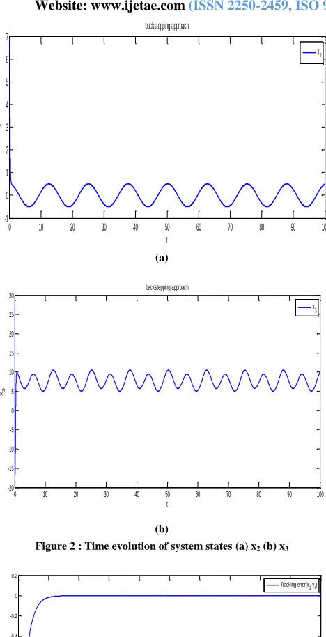
Figure 2 : Time evolution of system states (a) x2 (b) x3

Figure 3: Time evolution of tracking error

III. OBSERVER BASED CONTROLLER DESIGN FOR SYSTEM

OPERATION IN UNCERTAIN ENVIRONMENT

As discussed earlier, all the states of single link manipulator system with actuator dynamics in real practice are not always known. So, in order to provide full state feedback an observer is needed to be designed for unknown system states. Here, Luenberger observer structure has been presented to develop observer for uncertain environmental operations.

A.Proposed observer structure

The Luenberger observer for system mentioned in section 2 can be written as:

̂̇ ̂ ̂ ̂ ̂ ; (33)

The above system using suitably selected feedback controller ̂ leads to following dynamics

̂̇ A ̂+ ̂ ̂ (34)

where, observer output is taken as:

̂ ̂ (35)

Then tracking error „E‟ is:

= ̂ (36)

and the corresponding error dynamics can be written as

̇ ̂ (37)

In order to design an observer, the following assumptions must be made:

Assumption-1: The unknown parameters and states of the system are bounded and (A, C) pair is observable, with A as linear part of system dynamics and C is output matrix.

Assumption-2: The gain matrix 𝐿 satisfies the following condition:

(A-LC)TP+P (A-LC) = -Q ; (38)

where, A, B, C and L are system matrix, input matrix, output matrix and gain matrix, respectively and P and Q are positive matrices for observer system defined in equation (33).

Assumption-3: Nonlinearities of system follow Lipschitz conditions i.e.

̂ x - ̂

Where, is Lipschitz constant.

0 10 20 30 40 50 60 70 80 90 100

-1 0 1 2 3 4 5 6 7

t

x

2

x

2

0 10 20 30 40 50 60 70 80 90 100

-20 -15 -10 -5 0 5 10 15 20 25 30

t

x3

x₃

0 0.5 1 1.5 2 2.5 3 3.5 4 4.5 5

-1.4 -1.2 -1 -0.8 -0.6 -0.4 -0.2 0 0.2

time

Tr

a

c

k

in

g

e

rr

o

r

(5)

International Journal of Emerging Technology and Advanced Engineering

236

Consider Lyapunov function candidate for the error system in equation (37) as:

V = ETPE (39)

The time derivative of the Lyapunov function candidate is as follows:

̇ ̇ PE+ P ̇

̂ (40)

Using conditions of assumption (2) & (3), one can get

̇ x - ̂

‖ ‖( ) ‖ ‖ ‖ ‖ ‖ ‖ (41) Suitable selection of P as positive definite matrix and taking to be ( ) in assumption (2) and solving for suitable gains , equation (38) can be shown to be negative definite leading to the asymptotic stability of system. Hence, as time tends to infinity, error tends to zero leading to the desired behavior of the system.

B. Observer based backstepping approach

Let the observer system defined in equation (33) is required to track reference signal then tracking error is given by

= ̂- (42)

̇ = ̂ - ̇ (43)

Where, x2 is a fictitious control signal. Let desired signal

be then a new error variable is given by

= ̂ 𝐿 - (44) Let be chosen as:

= ̇ - 𝐿 (42)

This modifies equation (40) as:

̇= 𝐿 ̇ (45) The Lyapunov function candidate for stage one is chosen as:

= (46)

Making use of equation (40) and (43), we get:

̇ = - ; > 0 (47)

So the system is stabilized by the pseudo controller . From the definition of , error dynamics for second stage becomes:

̇ = ̂̇ - ̇ = ̂+ ̂ ̂ 𝐿 ̇ (48) Let, ̂ to be the fictitious control signal and be the desired value. Then, a new auxiliary error variable is defined as:

= ̂ (49) Now, equation (46) is modified as:

̇ ̂+ ̂ ̂ 𝐿 ̇ (50) Choosing desired value of next state to be

= (- ̂ – + ̇ 𝐿 ) (51)

It leads to:

̇ – ̂ (52)

Choosing Lyapunov function candidate for second stage as :

= + (53)

̇ = - + ( ̂+ ̂ ̂ - ̇ + 𝐿 )

̇ = - - ; , > 0 (54) For the last stage error dynamics is given by:

̇ ̂̇ ̇ (55)

Choosing Lyapunov function candidate for last stage as :

₍₅₆₎

̇ = - - + ̇

= - - + ̂ + ̂ ̂ 𝐿 ̇ (57)

System will be stable if and only if

̇ = - (58) Then,

̇ = - - - (59) Where, , > 0

(6)

International Journal of Emerging Technology and Advanced Engineering

237

̂ = ( ̇ - - ̂ 𝐿 ) (60)

Tracking error system can be written as:

̇= q (61) Where,

[

̂

]

(62)

For error system to converge, should be Hurwitz matrix. This can be achieved by pole placement technique. Using suitable positive values of gains K1, K2, K3 , above

error dynamics can be stabilized, hence leading to the desired tracking performance for the system under consideration.

C.Simulation results for observer based backstepping approach

Consider parameters for the manipulator system defined by equation (7) and (33) as

D=1, M=0.05, B=1, Km=10, H=0.5, N=10

Let the gains be selected as K1=15, K2= 25, K3=25 and

L1=K1 ; L2=K2 ; L3= K3 for simulation purpose. The initial

conditions are assumed as xo = [0.1, 6.28, 0, 0, 0, 0].

For present backstepping based observer case in uncertain environment, F1, F2, G1, G2are taken as per equation (3).

(a)

(b)

Figure 4: (a) Time evolution of system output y = , observer o/p

and reference signal & (b) expanded version of (a) in time span [0

5].

(a)

(b)

Figure 5: (a) Time evolution of x2 and ̂ & (b) expanded version of

(a) in time span [0 5].

0 10 20 30 40 50 60 70 80 90 100 0.5

1 1.5 2 2.5 3

y

r,

x

_

1

,x

1

^

t

refrence x1

x1^

0 0.5 1 1.5 2 2.5 3 3.5 4 4.5 5

0 0.5 1 1.5 2 2.5 3

y

r

,

x

_

1

,

x

1

^

t

refrence x₁ x1^

0 10 20 30 40 50 60 70 80 90 100

-1 0 1 2 3 4 5 6 7

t

x

_

2

,x

2

^

x₂ x2^

0 0.5 1 1.5 2 2.5 3 3.5 4 4.5 5

-1 0 1 2 3 4 5 6 7

t

x

_

2

,

x

2

^

[image:6.612.326.567.343.681.2]

(7)

International Journal of Emerging Technology and Advanced Engineering

238

(a)

(b)

Figure 6: (a) Time evolution of system state x3 and ̂ & (b) expanded

version of (a) in time span [0 5].

(a)

[image:7.612.55.285.131.465.2]

(b)

Figure 7: Time evolution of tracking errors& (b) expanded version of (a) in time span [0 5].

As it can be seen from the simulation result, observer based system converges faster than the former system. By comparing figure 3 and 7, we can see that tracking error becomes zero faster in later approach. The presented results show the efficacy of the proposed approach.

IV. CONCLUSION

Observers are the critical part of real world control system where all the states of the system are not known or not available for on line measurement. In this paper, design of controller for robot manipulator system using backstepping approach combined with Luenberger observer is presented for the robotic manipulator system with actuator dynamics. Simulation results for above mentioned approaches have been presented and compared. Simulation result shows the effectiveness of the proposed techniques.

REFERENCES

[1] Bastin G. and Gevers M., 1988, “Stable Adaptive Observers for

Nonlinear Time Varying Systems”, IEEE. Trans. on Automatic Control, vol. 33, no. 7, pp. 650-658.

[2] Gauthier J. P., Hammouri H. and S. Othman, 1992, “A simple

Observer for Nonlinear Systems Applications to Bioreactors”, IEEE. Trans. Automatic Control, vol. 37, no. 6, pp. 874-879.

[3] Khalil, H. 1996, Nonlinear Systems, New Jersey, Prentice Hall.

[4] Boutayeb M., Darouach M., and Rafaralahy H., 2002, “Generalized

state space observers for chaotic synchronization and secure communication,” IEEE Trans. Circuits Syst. I, Vol. 49, No. 3.

[5] Sharma B. B. and Kar I. N., 2011, “Observer-based synchronization

scheme for a class of chaotic systems using contraction theory”, Nonlinear Dynamics, vol. 63, no. 3, pp. 429–445.

0 10 20 30 40 50 60 70 80 90 100

-20 -10 0 10 20 30 40

t

x

_

3

,x

3

^

x3

x3^

0 0.5 1 1.5 2 2.5 3 3.5 4 4.5 5

-20 -10 0 10 20 30 40

t

x

_

3

,

x

3

^

x₃ x3^

0 10 20 30 40 50 60 70 80 90 100

-60 -50 -40 -30 -20 -10 0 10 20

Tr

a

c

k

in

g

e

rr

o

rs

time

e₁

e₂

e₃

0 0.5 1 1.5 2 2.5 3 3.5 4 4.5 5

-60 -50 -40 -30 -20 -10 0 10 20

Tr

a

c

k

in

g

e

r

o

r

s

time

[image:7.612.330.561.145.291.2]

(8)

International Journal of Emerging Technology and Advanced Engineering

239

[6] Morgul O. and Solak E., 1996, “Observer based synchronization of

chaotic systems,” Phys. Rev. E., vol. 54, pp. 4802–4811.

[7] Grassi, G. and Mascolo S., 1997, “Nonlinear observer design to

synchronize hyperchaotic systems via a scalar signal”, IEEE Trans. Circuits Syst.-I, vol. 44, no. 10, pp. 1011–1014.

[8] Meena N., Sharma B. B., “Backstepping Algorithm with Sliding

Mode Control for Magnetic Levitation System”, International Journal of Emerging Trends in Electrical and Electronics, vol. 10, pp. 39-43, 2014.

[9] Agrawal V. and Sharma B. B., 2014, “An observer based approach

for multi-scroll chaotic system synchronization and secure communication with multi-shift ciphering”, Int. Conf. on Advances in Engineering and Technology Research (ICAETR), pp.1-6.

[10] Sharma V, Agrawal V, Sharma B B and Nath R, 2016, “Unknown

input nonlinear observer design for continuous and discrete time systems with input recovery scheme”, Nonlinear Dynamics, pp.

1-14, 2016, DOI: 10.1007/s11071-016-2713-5

[11] Lam H. K. and Li H., 2013, “Output-feedback tracking control for

polynomial fuzzy-model-based control systems”, IEEE transactions on industrial electronics, vol. 60, no. 12.

[12] Huang H., Yan J., and Cheng T. , 2007, “Development and fuzzy

control of a pipe inspection robot,” IEEE Trans. Ind. Electron., vol. 57, no. 3, pp. 1088– 1095, [13] Liu Y. J. and Wang W., “Adaptive fuzzy control for a class of uncertain nonaffine nonlinear systems,” Inf. Sci., vol. 177, no. 18, pp. 3901–3917.

[13] Tong S. and Li Y., 2009, “Observer-based fuzzy adaptive control for

strict feedback nonlinear systems,” Fuzzy Sets Syst., vol. 160, no. 12, pp. 1749– 1764.

[14] J. J. Slotine, S. S. Sastry, 1983, “Tracking control of non-linear

systems using sliding surfaces, with application to robot manipulators”, International Journal of Control, Vol. 38, no. 2.

[15] Krstic M., Kanellakopoulos I. and Kokotovic P., 1995, “Nonlinear

and Adaptive Control Design” John Wiley and sons, New York.

[16] Murray R. M., Li Z .and Sastry S. S., 1993, “A mathematical

introduction to robot manipulation”, CRC Press.

[17] Dochain, D. and Perrier, M., 2003, “Adaptive Backstepping