Munich Personal RePEc Archive
Noncausality and Asset Pricing
Lof, Matthijs
8 April 2011
Online at
https://mpra.ub.uni-muenchen.de/30519/
öMmföäflsäafaäsflassflassflas
fffffffffffffffffffffffffffffffffff
Discussion Papers
Noncausality and Asset Pricing
Matthijs Lof
University of Helsinki and HECER
Discussion Paper No. 323
April 2011
ISSN 1795-0562
HECER
Discussion Paper No. 323
Noncausality and Asset Pricing*
Abstract
Misspecification of agents' information sets or expectation formation mechanisms may
lead to noncausal autoregressive representations of asset prices. Annual US stock prices
are found to be noncausal, implying that agents' expectations are not revealed to an
outside observer such as an econometrician observing only realized market data. A
simulation study shows that noncausal processes can be generated by asset-pricing
models featuring heterogeneous expectations.
JEL Classification:
C58, D84, G12, G17
Keywords:
noncausal autoregressions, stock prices, heterogeneous expectations.
Matthijs Lof
Department of Political and Economic Studies
University of Helsinki
P.O. Box 17 (Arkadiankatu 7)
FI-00014 University of Helsinki
FINLAND
e-mail:
[email protected]
1
Introduction
Recent research (e.g. Lanne and Saikkonen, 2011a,b) finds that many financial and economic
vari-ables are noncausal, in the sense that current observations seem to depend on both past and future
realizations, rather than only on past realizations. This paper discusses noncausality of asset prices
and dividends. Recent literature dealing with noncausality focuses mainly on econometric issues,
such as instrument selection in GMM estimation (Lanne and Saikkonen, 2011a) and forecasting
(Lanne et al., 2010, 2011). In this paper the focus is not on empirical implications but rather on the
economic interpretation of noncausality. I show by simulation that noncausality can be generated
by excluding relevant information from the econometric model. Asset prices are shown to be
non-causal when the econometric model is based on observed market data, but fails to include the correct
expectation formation mechanism.
A noncausal autoregressive (AR) process differs from a conventional causal AR process in the
dependence on both future and past errors, implying that future errors are predictable given the
realized observations of the variable in question. An early discussion of noncausal autoregressions
is provided by Breidt et al. (1991). Recently, Lanne and Saikkonen (2011b) introduced a useful
reparametrization of the noncausal AR process that allows for explicit dependence on both leads
and lags of the variable in question. A stationary noncausal AR(r,s) processyt, depending onrlags
andsleads, is defined by:
φ(L)ϕ(L−1)yt=εt, (1)
withφ(L) =1−φ1L−...φrLr,ϕ(L−1) =1−ϕ1L−1−...ϕrL−s,εt ∼i.i.d.(0,σ2)andLis a standard
lag operator (Lkyt =yt−k). Both polynomials have their roots outside the unit circle. If ϕj6=0,
for some j∈ {1, ..,s}, (1) is a noncausal process, which may be referred to as purely noncausal if
φ1=...=φp=0. Whenytis a vector, (1) defines a noncausal vector autoregressive process VAR(r,s)
(Lanne and Saikkonen, 2009).
well known that any stationary causal AR(r,0) process has a backward-looking MA representation:
yt=φ(L)−1εt =
∞
∑
j=0
ψjεt−j.
The MA representation of a noncausal AR(r,s) process is, on the other hand, both backward- and
forward-looking:
yt =ϕ(L−1)−1φ(L)−1εt =
∞
∑
j=−∞ ψjεt−j,
while a purely noncausal AR(0,s) process even has a purely forward-looking MA representation:
yt =ϕ(L−1)−1εt=
∞
∑
j=0
ψjεt+j.
A noncausal process can not be inverted into a backward-looking MA representation, meaning that
the errors are nonfundamental. Nonfundamentalness arises when the agents in the economy base
their expectations on a larger information set than the information set available to an econometrician,
in which case the residuals from the estimated autoregression are not an interpretable function of
the true shocks to the agents’ information (Hansen and Sargent, 1991; Alessi et al., 2011). In this
situation, a noncausal autoregression may fit the data better, because it takes the omitted information
into account, by allowing for predictable errors, even without explicit specification of the correct
information set (Lanne and Saikkonen, 2011b).
The agents’ information set is a flexible concept. The most obvious example of an
econometri-cian having a smaller information set than the agents in the economy is the omission of one or more
relevant decision variables from the estimated model. In this paper, I argue that another example
of such a situation occurs when the econometrician and the agents observe the same variables, but
the econometrician misunderstands the complexity of the expectation formation mechanism, by
es-timating a linear model while the true mechanism is nonlinear. In section 3, I show that noncausality
is often observed when a linear univariate autoregressive model is estimated for a variable that was
In section 4, the existence of heterogeneous beliefs is shown to be a possible source of
non-causality of asset prices. In this case, different agents form different expectations about the future,
making it difficult for an econometrician to observe or infer these expectations. This is an important
missing piece of information, since on financial markets these expectations ultimately drive asset
prices.
To motivate the search for sources of noncausality in asset pricing, the next section presents
empirical evidence that historical US stock prices are indeed noncausal.
2
Empirical results
To determine whether a causal or noncausal autoregression fits a certain variableyt better, I will
follow the model selection procedure proposed by Lanne and Saikkonen (2011b). First, a causal
autoregression AR(p) is estimated by least squares to find the optimal number of lags psuch that
the model seems adequate in describing the autocorrelation. In this paper the number of lags is
selected by the Bayesian Information Criterion (BIC). Next, model (1) is estimated by maximum
likelihood for all possible combinations ofrandsfor whichr+s=p. After estimating all possible
AR(r,s) models, the specification yielding the largest value of the likelihood function is chosen as
the adequate autoregression. If for this models>0, the variable yt is referred to as noncausal.
Since causal and noncausal autoregressive processes are indistinguishable when the error terms are
Gaussian, another distribution needs to be assumed (Breidt et al., 1991). With macro-economic
and financial time series this does not need to be a problem, since Gaussianity if often rejected for
these time series due to fat tails. Therefore, t-distributed errors are assumed. Details on maximum
likelihood estimation of the noncausal autoregressive model with t-distributed errors are provided
by Lanne and Saikkonen (2009, 2011b) for both univariate and multivariate processes.
This model selection procedure is applied to univariate and bivariate time series related to asset
pricing, using long-term data on the US stock market provided by Shiller (2005). This dataset
average dividends (Dt) paid to investors holding shares in this index. Noncausality is checked for the
log-difference of prices (△pt=log(Pt)−log(Pt−1)) and dividends (△dt =log(Dt)−log(Dt−1)), as
well as for the bivariate processes(△pt,△dt)′and(δt,△dt)′, withδt=log(Pt/Dt)is the log
price-dividend (PD) ratio. Table 1 depicts the log-likelihood values for all estimated AR(r,s) models.
Log-differenced dividends are found to be causal, but log-differenced prices and both VARs are best
described by noncausal processes.
TABLE 1
△pt △dt (δt,△dt)′ (△pt,△dt)′
(r,s) L (r,s) L (r,s) L (r,s) L
(1,0) 41.8 (1,0) 123.3 (2,0) -240 (1,0) -360
(0,1) 42.8 (0,1) 119.9 (1,1) -228 (0,1) -350
(0,2) -229
JB 0.01 0.00 0.00 0.00
LB 0.08 0.20 0.19 0.22 0.13 0.27
MLL 0.36 0.12 0.11 0.06 0.08 0.06
Notes: Log-likelihood values for all possible AR(r,s) specifications such that p=r+s. The specification that maximizes the log-likelihood for each variable is depicted in bold. The lag lengthpis selected by the BIC, based on a causal Gaussian AR, after which Gaussianity of the residuals is tested with a Jarque-Bera test. JB refers to the p-value of this test. LB and MLL refer to the p-values of the Ljung-Box and McLeod-Li tests (5 lags), applied to the residuals of the optimal (non)causal t-distributed AR.
Table 1 further shows some diagnostic test results. After selecting the number of lags pbased on a
Gaussian causal AR, Gaussianity of the residuals is tested. Gaussianity is rejected by a Jarque-Bera
test for all ARs, justifying estimation by non-Gaussian maximum likelihood. The residuals of the
au-toregression selected as adequate are furthermore subjected to tests for autocorrelation (Ljung-Box)
and conditional heteroscedasticity (McLeod-Li). There is no evidence for remaining autocorrelation
or heteroscedasticity at the 5% level. In general, the selected noncausal autoregressions seem to
describe these time series well.
The VAR including PD ratios and dividends(δt,△dt)′ was proposed by Campbell and Shiller
result that(δt,△dt)′ is noncausal is consistent with findings by Lanne and Saikkonen (2009), who
show that the VAR proposed by Campbell and Shiller (1987) to model the expected term spread
of interest rates is also noncausal. Noncausality of(δt,△dt)′ implies that agents do not base their
expectations only on lags of the PD ratio and the dividend growth rate. The same argument applies to
the second VAR in Table 1, including the growth rates of prices and dividends(△pt,△dt)′. Taking
expectations conditional on all information datedt−1 and earlier shows that these expectations can
not be expressed as a function of observable data alone:
Et−1
δt
△dt
= Φ1
δt−1 △dt−1
+Π1Et−1
δt+1 △dt+1
+Et−1
ε1,t
ε2,t
Et−1
△pt
△dt
= Π1Et−1
△pt+1 △dt+1
+Et−1
ε1,t
ε2,t
.
An economic interpretation of noncausality is therefore that agents’ expectations are not revealed
when only realized prices and dividends are observed. Future realizations or a wider information set
are required to infer the true expectations. This observed dependence on leading observations may
be caused by misspecification of the agents’ information set. This issue is further discussed in the
remainder of this paper.
3
Misspecified autoregressions
I illustrate that misspecification of the econometric model can cause noncausality by simulating two
simple AR processes. In the first example the variable of interest is generated by a multivariate
process, but estimated as a univariate process. In the second example the data generating process is
nonlinear, while a linear model is estimated.
bivariate process: xt yt = a b 0 c
xt−1
yt−1
+
εx,t
εy,t
εx,t,εy,t ∼t3(0,1). (2)
The errorsεx,t andεy,t are independent and t-distributed with three degrees of freedom, zero mean
and variance one. I calibratea=c=0.8 and generate 200 observations ofxt andyt for different
values ofb.After this simulation,yt is dropped from the information set andxt is estimated as a
uni-variate AR process to check noncausality by the model selection procedure discussed in the previous
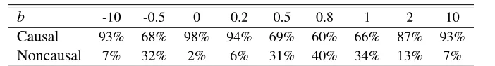
section. This simulation is repeated 5000 times. Table 2 shows how often the model selection
proce-dure selects causal and noncausal representations for different values ofb.1 Whenb=0, the causal
autoregression is the correct specification and is selected in 98% of the simulations. However, when
b6=0,xt is driven by two shocksεx,t andεy,t, while only one shock can be identified by estimating
an autoregression. Due to this nonfundamentalness, a noncausal autoregression is selected as the
adequate specification more often, up to 40% of the simulations forb=0.8. Interestingly, when
b becomes larger in absolute value, εy,t becomes the dominant shock and the causal AR is again
selected more often. In the case thatb=10, the contribution ofεx,t to the dynamics ofxt, relative
to the contribution ofεy,t, is so small that the true process can be well approximated by a causal AR
[image:9.612.135.486.529.576.2]process with only one shock.
TABLE 2
b -10 -0.5 0 0.2 0.5 0.8 1 2 10
Causal 93% 68% 98% 94% 69% 60% 66% 87% 93%
Noncausal 7% 32% 2% 6% 31% 40% 34% 13% 7%
Notes: Percentage of causal and noncausal outcomes of the AR forxt after 5000 simulations of model (2), with
a=c=0.8and different values ofb. The sample size in each simulation is 200 observations.
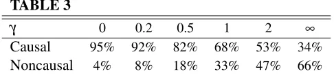
Next, a univariate nonlinear Logistic Smooth Transition Autoregressive (LSTAR) process is
gener-ated:
yt=α1yt−1(1−G(st−1)) +α2yt−1G(st−1) +εt
G(st−1) = (1+exp[−γst−1])−1
εt ∼t3(0,1). (3)
This process is a weighted average of two causal AR(1) regimes. Since the weights are time-varying,
the process is nonlinear. However whenγ=0, the transition functionG(st−1) =1/2in all periods,
so the process is linear. On the other hand, when γ =∞, G(st−1) is either zero or one, meaning
the process reduces to a Threshold Autoregressive (TAR) process. In short, the process becomes
more nonlinear whenγ increases. I choose the transition variablest−1=△yt−1and the calibration
α1=0.8 andα2=−0.2, so that each regime is stationary and differs considerably from the other
regime. A sample of 200 observations is simulated for different values ofγ: 0, 0.2, 0.5, 1, 2 and
10.000(≈∞), after which a linear AR model is fitted to the data to check for noncausality. Table
3 displays the results of 5000 repetitions. In the linear case (γ =0), a noncausal specification
is selected in 4% of the simulations. However, the number of noncausal representations selected
steadily increases withγ, up to 66% of the simulations for the TAR model. These results show that
not only after omitted variables, but also after misspecification of the functional form, a noncausal
process often approximates the true process better than a causal process, even if these processes
[image:10.612.185.428.519.573.2]depend by no means on the future.
TABLE 3
γ 0 0.2 0.5 1 2 ∞
Causal 95% 92% 82% 68% 53% 34%
Noncausal 4% 8% 18% 33% 47% 66%
Notes: Percentage of causal and noncausal outcomes of the AR foryt after 5000 simulations of model (3),with
4
Heterogeneous expectations
Returning to asset pricing, the results of the previous section suggest that the observed noncausality
in Table 1 could be the result of the misspecification of agents’ expectation formation mechanisms:
Agents participating in the stock market base their expectations on more information than past prices
and dividends alone and/or their expectations are a nonlinear function of the available information.
The existence of heterogeneous beliefs is a natural candidate for such a situation. Kasa et al.
(2010) derive conditions under which informational heterogeneity (agents receiving different signals
about future dividends) imposes agents to forecast the forecasts of other agents, as in Townsend
(1983), which leads to a nonrevealing equilibrium. Kasa et al. (2010) explicitly show how the
process of prices and dividends is under these conditions not invertible into a backward-looking
moving average process (i.e. is nonfundamental) and argue that an econometrician who does not
observe these different signals will misinterpret the residuals from a VAR as shocks to the agents’
information.
To check what type of investor behavior generates noncausality, I simulate asset prices under
different expectation regimes. I consider a representative-agent model and two models featuring
boundedly rational agents with heterogeneous beliefs. After each simulation, I act as an
econome-trician who does not understand the structure of the underlying model and estimate both causal and
noncausal VARs for prices and dividends, to find out which VAR fits the data best. The starting point
for this simulation exercise are the dividends, which are assumed to be exogenous, not depending
on asset prices. To be precise, dividends are generated by a causal AR(1) process:
dt =α1+α2dt−1+εt, (4)
with εt ∼t3(0,σε2). The fundamental value p∗t of the asset equals the sum of all expected future
p∗t =
∞
∑
i=0
Et−1[dt+i]
(1+r)i
Et−1[dt+i] = α1+α2Et−1[dt+i−1].
(5)
In a world where all agents have rational and homogeneous beliefs about the future (i.e. a rational
representative-agent model) the asset price should reflect the expected fundamental value of the
asset:
pt =pt∗+ηt ηt ∼t3(0,ση2). (6)
The i.i.d. error term ηt is added so that pt is not an exact linear function of dt−1, which would
make the parameters in a VAR including prices and dividends not identifiable. The error term can
however be justified as noise due to frictions, the existence of noise traders or minor uncertainties
about fundamentals.
A more general model relaxes the assumptions of homogeneity and rationality and allows for
heterogeneous beliefs. I follow the asset-pricing model proposed by Brock and Hommes (1998),
featuring many types of boundedly rational agents who form different beliefs about the future. With
Hdifferent types of agents, asset prices are determined by the following equation:
pt = H
∑
h=1
nh,tEh,t−1[pt+1+dt+1]
1+r +ηt, (7)
whereEh,t(·)represents the expectation formation mechanism of agent typehandnh,t is the fraction
of the population behaving according to typehat timet. In the special case thatH=1 andE1,t(·)
denotes rational expectationsEt(·), (7) reduces to (6). To introduce heterogeneous beliefs it is useful
to formulate (7) in deviation from the fundamental value:
xt = H
∑
h=1
nh,tfh,t
1+r +ηt, (8)
with xt =pt−pt∗ is the realized difference from the fundamental value and fh,t =Eh,t−1[pt+1]−
Et−1
p∗t+1
funda-mental value, but disagree on the dynamics of the deviation from the fundafunda-mental value. In
particu-lar, each type applies linear prediction rules based on lagged prices to form their expectations:
fh,t =ghxt−1+bh. (9)
The fraction of each type, nh,t, varies over time according to evolutionary dynamics. The type of
agent that realizes a high profit from trading in the previous period will become more influential in
the next period:
nh,t=
exp(βUh,t−1)
H
∑
i=1
exp(βUi,t−1)
, (10)
whereUh,t = (xt−(1+r)xt−1)(fh,t−1−(1+r)xt−2)−ch denote the realized profits for each type,
such that the fractions of all types add up to one. A full derivation of these equations is provided
in Brock and Hommes (1998). These evolutionary dynamics are comparable to the ’forecasting the
forecasts of others’ property considered by Townsend (1983) and Kasa et al. (2010): Agents do
not commit only to their own beliefs, but take into consideration the expectations of other agents,
knowing that the expectations of others have a direct effect on asset prices. The parameterβ defines
the willingness or capability of agents to switch to another strategy. I now consider an example with
two different agent types: The first type is the fundamentalist, who believes deviations from the
fundamental value should disappear:
fF,t=0. (11)
The other type is the chartist or trend-follower, who believes deviations from the fundamental value
in the previous period will persist:
fC,t =gCxt−1. (12)
The parametergC defines the difference between the behavior of the agents. WhengC=0 , both
value should disappear over time, but they disagree about the pace of this correction. In Brock and
Hommes (1998) and in this papergC≥1+r, meaning the chartists believe that the asset price will
diverge from the fundamental value. Fundamentalists will therefore buy stocks when the price is
under its fundamental valuation and sell when it is above. Chartists act the other way around which
may create both positive and negative stock price bubbles even in the absence of random shocks
(Brock and Hommes, 1998). Chartists are commonly thought of as technical traders, although Parke
and Waters (2007) argue that similar behavior could be observed when agents experiment with
different information sets to form expectations. The representative-agent benchmark (6) is nested
in the model with fundamentalists and chartists (7-12): The models can be made identical either by
settinggC=0, ornF,t =1∀t.
A final example includes two other types: Optimists and pessimists (or bulls and bears). The
optimist type forms expectations with a positive bias, while the pessimist type forms expectations
with a negative bias:
fO,t = b
fP,t = −b,
(13)
withb≥0. This model is identical to the representative-agent benchmark (6) ifb=0. Optimists
believe the asset is undervalued while pessimists believe the asset is overvalued. This disagreement
could be the result of heterogeneous information on the fundamentals: The optimists (pessimist)
receives positive (negative) signals about future fundamentals, although also other factors such as
different levels of risk-aversion could cause the different beliefs.
I simulate dividends (4) and asset prices according to the representative-agent model (6), the
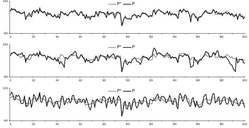
fundamentalist-chartist model (7-12) and the optimist-pessimist model (7-10,13). Plots of 200
sim-ulated observations of the asset prices under each regime are given in Figure 1, together with the
calibration of the parameters. The calibration of the profit functions and switching probabilities (10)
as well as the behavioral parameters of the chartists and fundamentalists is identical to the
2.5% of the average fundamental value. Figure 1 shows that under the representative-agent model,
the difference between the fundamental values and the realized price is i.i.d. random noise (top
panel). With the fundamentalist-chartist model, longer lasting deviations are observed. Thinking of
annual data, the middle panel shows several examples of stock price bubbles lasting up to a decade.
Finally, the bottom panel of Figure 1 shows the optimist-pessimist model, with continuous cycles of
overvaluation followed by undervaluation lasting just a couple of years.
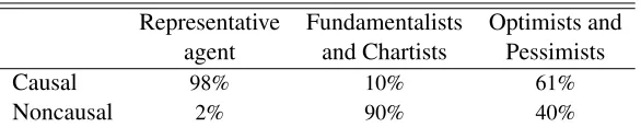
After each simulation, the model selection procedure described in section 2 is applied to
deter-mine whether the VAR including (demeaned) prices and dividends(pt,dt)′ is causal or noncausal.
Since dividends follow a stationary AR process, there is no need to take (log) differences. This
simulation is repeated 5000 times. Table 4 shows how often causal and noncausal specifications are
selected for each model..
190 240
0 20 40 60 80 100 120 140 160 180 200
P* P
190 240
0 20 40 60 80 100 120 140 160 180 200
P* P
190 240
0 20 40 60 80 100 120 140 160 180 200
[image:15.612.92.516.367.586.2]P* P
Figure 1: Simulated asset prices. Fundamental values and realized prices generated by: Representative agent
(Top panel), Fundamentalists and Chartists(Middle panel) and Optimists and Pessimists(Bottom panel). Cal-ibration: α1=4,α2=0.8,σε2=1,r=0.1,ση2 =2,β =3.6, gC=1.2,cF =1,cC=cO=cP =0,
TABLE 4
Representative Fundamentalists Optimists and agent and Chartists Pessimists
Causal 98% 10% 61%
Noncausal 2% 90% 40%
Notes: Percentage of causal and noncausal outcomes of the VAR for (pt,dt)′ after 5000 simulations with a
representative-agent model and with heterogeneous-agents models. The sample size in each simulation is 200 observations.
With a representative agent the VARs of prices and dividends are found to be almost exclusively
causal. However, with the optimist-pessimist model noncausality is found for almost 40% of the
simulations and with the fundamentalist-chartist model even in 90% of the simulations, even though
all types of agents considered are fully backward-looking in the sense that they base their decisions
only on past prices and dividends. These results confirm that heterogeneous beliefs are a potential
source of noncausality. This is consistent with the simulation results in section 3, since the switching
between strategies causes nonlinearity in the prices, even if all beliefs are linear functions of realized
data. Moreover, the fractions of each type of agent in the population can also be interpreted as
an omitted variable. Parke and Waters (2007) note that asset prices are generated by a process
Pt= f(Ωt−1,nt,εt), whereΩt−1includes all past prices and dividends andnt include the fractions of
each type. In this case an econometrician will have access toΩt−1, but can not observe behavior or expectations. An estimated model will therefore be of the formPt = fˆ(Ωt−1,εˆt), so thatnt is an
omitted variable.
5
Conclusions
This paper presents empirical results confirming that several autoregressions related to asset
pric-ing are noncausal. A simulation study shows that nonlinearity caused by heterogeneous beliefs is
a potential source of noncausality. This is an example of the econometrician having a smaller
observed, an important piece of information about the asset pricing process is omitted, namely the
expectations and fractions of each type of agent.
Investor heterogeneity is not the only potential source of noncausality. A representative agent
model may also be nonlinear, because of a time-varying (stochastic) discount factor. Moreover, in
reality dividends are generated by a more complicated process than an AR(1) process and depend on
many other variables. When markets are efficient, agents will rationally use all available information
to form expectations about the future, making it nearly impossible for an econometrician to create a
dataset that can replicate these expectations. Both these cases could potentially generate noncausal
asset prices.
References
Alessi, L., M. Barigozzi, and M. Capasso: 2011, ‘Nonfundamentalness in Structural Econometric
Models: A Review’. International Statistical Review(forthcoming).
Breidt, F. J., R. A. Davis, K.-S. Lh, and M. Rosenblatt: 1991, ‘Maximum likelihood estimation for
noncausal autoregressive processes’. Journal of Multivariate Analysis36(2), 175–98.
Brock, W. A. and C. H. Hommes: 1998, ‘Heterogeneous beliefs and routes to chaos in a simple asset
pricing model’. Journal of Economic Dynamics and Control22(8-9), 1235–1274.
Campbell, J. Y. and R. J. Shiller: 1987, ‘Cointegration and Tests of Present Value Models’. Journal
of Political Economy95(5), 1062–88.
Campbell, J. Y. and R. J. Shiller: 1988, ‘The Dividend-Price Ratio and Expectations of Future
Dividends and Discount Factors’. Review of Financial Studies1(3), 195–228.
Hansen, L. P. and T. J. Sargent: 1991, ‘Two Difficulties in Interpreting Vector Autoregressions’. In:
L. P. Hansen and T. J. Sargent (eds.):Rational Expectations Econometrics. Westview Press, Inc.,
Kasa, K., T. B. Walker, and C. H. Whiteman: 2010, ‘Heterogeneous Beliefs and Tests of Present
Value Models’. Unpublished manuscript.
Lanne, M., A. Luoma, and J. Luoto: 2011, ‘Bayesian Model Selection and Forecasting in Noncausal
Autoregressive Models’. Journal of Applied Econometrics(forthcoming).
Lanne, M., J. Luoto, and P. Saikkonen: 2010, ‘Optimal Forecasting of Noncausal Autoregressive
Time Series’. HECER Discussion Paper 286.
Lanne, M. and P. Saikkonen: 2009, ‘Noncausal vector autoregression’. Research Discussion Papers
18/2009, Bank of Finland.
Lanne, M. and P. Saikkonen: 2011a, ‘GMM Estimation with Noncausal Instruments’. Oxford
Bul-letin of Economics and Statistics(forthcoming).
Lanne, M. and P. Saikkonen: 2011b, ‘Noncausal Autoregressions for Economic Time Series’.
Jour-nal of Time Series Econometrics(forthcoming).
Parke, W. R. and G. A. Waters: 2007, ‘An evolutionary game theory explanation of ARCH effects’.
Journal of Economic Dynamics and Control31(7), 2234–2262.
Shiller, R. J.: 2005,Irrational exuberance. Princeton University Press.
Townsend, R. M.: 1983, ‘Forecasting the Forecasts of Others’. Journal of Political Economy91(4),