Spatio temporal variability of snow water equivalent in the extra tropical Andes Cordillera from distributed energy balance modeling and remotely sensed snow cover

www.hydrol-earth-syst-sci.net/20/411/2016/ doi:10.5194/hess-20-411-2016

© Author(s) 2016. CC Attribution 3.0 License.

Spatio-temporal variability of snow water equivalent in the

extra-tropical Andes Cordillera from distributed energy

balance modeling and remotely sensed snow cover

E. Cornwell1, N. P. Molotch2,3, and J. McPhee1,4

1_{Advanced Mining Technology Center, Facultad de Ciencias Físicas y Matemáticas, Universidad de Chile, Santiago, Chile} 2_{Department of Geography and Institute of Arctic and Alpine Research, University of Colorado, Boulder, USA}

3_{Jet Propulsion Laboratory, California Institute of Technology, Pasadena, California, USA}

4_{Departamento de Ingeniería Civil, Facultad de Ciencias Físicas y Matemáticas, Universidad de Chile, Santiago, Chile} Correspondence to: J. McPhee ([email protected])

Received: 3 July 2015 – Published in Hydrol. Earth Syst. Sci. Discuss.: 3 September 2015 Revised: 8 December 2015 – Accepted: 24 December 2015 – Published: 25 January 2016

Abstract. Seasonal snow cover is the primary water source for human use and ecosystems along the extratropical Andes Cordillera. Despite its importance, relatively little research has been devoted to understanding the properties, distribu-tion and variability of this natural resource. This research provides high-resolution (500 m), daily distributed estimates of end-of-winter and spring snow water equivalent over a 152 000 km2 domain that includes the mountainous reaches of central Chile and Argentina. Remotely sensed fractional snow-covered area and other relevant forcings are combined with extrapolated data from meteorological stations and a simplified physically based energy balance model in order to obtain melt-season melt fluxes that are then aggregated to estimate the end-of-winter (or peak) snow water equivalent (SWE). Peak SWE estimates show an overall coefficient of determinationR2of 0.68 and RMSE of 274 mm compared to observations at 12 automatic snow water equivalent sensors distributed across the model domain, withR2values between 0.32 and 0.88. Regional estimates of peak SWE accumula-tion show differential patterns strongly modulated by eleva-tion, latitude and position relative to the continental divide. The spatial distribution of peak SWE shows that the 4000– 5000 m a.s.l. elevation band is significant for snow accumu-lation, despite having a smaller surface area than the 3000– 4000 m a.s.l. band. On average, maximum snow accumula-tion is observed in early September in the western Andes, and in early October on the eastern side of the continental di-vide. The results presented here have the potential of

inform-ing applications such as seasonal forecast model assessment and improvement, regional climate model validation, as well as evaluation of observational networks and water resource infrastructure development.

1 Introduction

re-sources. This research presents the first spatially and tem-porally explicit high-resolution SWE reconstruction over the snow-dominated extratropical Andes of central Chile and Ar-gentina based on a physical representation of the snowpack energy balance (Kustas et al., 1994) and remotely sensed snow extent (Dietz et al., 2012) between years 2001 and 2014. A key advantage of the presented product is its in-dependence from notoriously scarce and unreliable precip-itation measurements at high elevations. Estimates of maxi-mum SWE accumulation and depletion curves are obtained at 500 m resolution, coincident with the MODIS MOD10A1 Fractional Snow Cover product (Hall et al., 2002).

Patterns of hydroclimatic spatio-temporal variability in the extratropical Andes have been studied with increased inten-sity over the last couple of decades, as pressure for water resources has mounted while at the same time rapid changes in land use and climate have highlighted the societal need for increased understanding of water resource variability and trends under present and future climates. The vast majority of studies have relied on statistical analyses of instrumen-tal records and regional climate models to present synoptic-scale summaries of precipitation (e.g., Aravena and Luck-man, 2009; Falvey and Garreaud, 2007; Garreaud, 2009), temperature (Falvey and Garreaud, 2009), snow accumu-lation (Masiokas et al., 2006) and streamflow variability (Cortés et al., 2011; Núñez et al., 2013). Currently, no high-resolution, large-scale distributed assessments of snow water equivalent are available for the Andes region.

The SWE reconstruction method seeks to estimate end-of-winter accumulation by back accumulating melt energy fluxes during the depletion season. The methods and assump-tions required for SWE reconstruction have been tested and refined since initial development (Cline et al., 1998). Ap-plications across a variety of scales have been presented in recent years. In the Sierra Nevada, Jepsen et al. (2012) compared SWE reconstructions to distributed snow surveys in a 19.1 km2 basin (R2=0.79), while Guan et al. (2013) obtained good correlation with SWE observations from an operational snow sensor network across the entire Sierra Nevada (R2=0.74). In the Rocky Mountains, Jepsen et al. (2012) obtained anR2value of 0.61 when comparing re-constructed SWE to spatial regression from snow surveys, and Molotch (2009) estimated SWE with a mean absolute error (MAE) of 23 % compared to intensive study areas. A useful discussion on the uncertainties of the SWE recon-struction method – albeit one based on temperature-index melt equations – was presented by Slater et al. (2013), who demonstrated that errors in forcing data are at least, if not more, important than snow-covered area data availability. The vast majority, if not all, of SWE reconstruction exercises have been developed in the northern hemisphere, under en-vironmental conditions quite different from those predomi-nant in the extratropical Andes Cordillera. Here, snow dis-tribution and properties have been analyzed in a few local studies (e.g., Ayala et al., 2014; Cortés et al., 2014b;

Gas-coin et al., 2013), but no large-scale estimations at a rele-vant temporal and spatial resolution for hydrologic applica-tions have been presented. In fact, the Andes of Chile and Argentina display near-ideal conditions for the SWE recon-struction approach due to (1) the near absence of forest cover over a large fraction of the domain where snow accumula-tion is hydrologically significant; (2) the sharp climatolog-ical distinction between wet (winter: June through August) and dry (spring/summer: September through March) seasons, with most of annual precipitation falling during the former; and (3) the low prevalence of cloudy conditions during the spring and summer months over the mountains, which afford a high availability of remotely sensed snow cover informa-tion. Conversely, the SWE reconstruction presented here is certainly subject to a series of uncertainty sources, such as the sparseness of the hydrometeorological observational net-work, which limits both the availability of forcing and vali-dation data.

However, this is the first estimation of peak SWE and snow depletion distribution at this scale and spatial resolution for the extratropical Andes, and the information shown here can be useful for several applications such as understanding year-to-year differential accumulation patterns that may impact the performance of seasonal streamflow forecast models that rely on point-scale data only. Also, the SWE reconstruction can be used to validate output from global or regional cli-mate models and reanalysis, which are being increasingly employed to estimate hydrological states and fluxes in un-gauged regions. By analyzing the spatial correlation of snow accumulation and hydrometeorological variables, distributed SWE estimates can inform the design of improved climate observation networks. Likewise, from analyzing the obtained SWE estimates in light of the necessary modeling assump-tions and data availability we are able to highlight future re-search directions aimed at quantifying and reducing these un-certainties.

The objectives of this research include the following: (1) to assess the dominant patterns of spatio-temporal variability in snow water equivalent of the snow-dominated extratropical Andes Cordillera; and (2) to explicitly evaluate the strengths and weaknesses of the SWE reconstruction approach in dif-ferent sub-regions of the extratropical Andes using snow sen-sors and distributed snow surveys.

2 Study area

popula-Figure 1. Study area and model domain: (a) river basins, stream

gages (red circles) and sites where snow survey data are available (green circles); (b) hydrologic units (C1 to C8) and snow-pillow stations (white circles).

tion (http://www.ine.cl) as well as most of the country’s agricultural output, hydropower and industrial activities. In the case of Argentina, 7 % of the population is located in the provinces of La Rioja, San Juan, Mendoza and north-ern Neuquén (http://www.indec.gov.ar/), with primary wa-ter uses in agriculture and hydropower. The selected wawa-ter- water-sheds have unimpeded streamflow observations and a snow-dominated hydrologic regime (Fig. 2). River basins included in this study have been grouped in eight clusters, or hydro-logic response units, based on the seasonality of river flow, numbered C1 to C8 in Fig. 1b. Due to differences in topog-raphy and locations of stream gages, the number of headwa-ter basins contained within clusheadwa-ters differs markedly on both

Figure 2. Summarized hydro-climatology of the model domain.

Data from meteorological stations located within zones C1, C4, C3 and C8 summarized the hydro-climatological regime of the north-western, northeastern, southwestern and southeastern zones, respec-tively. Total SWE is SWE measured at selected snow-pillow sta-tions.

sides of the cordillera, with larger watersheds on the Argen-tinean side.

The hydro-climate is mostly controlled by orographic ef-fects on precipitation (Falvey and Garreaud, 2007) and inter-annual variability associated with the Pacific Ocean through the El Niño–Southern Oscillation and Pacific Decadal Oscil-lation (Masiokas et al., 2006; Newman et al., 2003; Rubio-Álvarez and McPhee, 2010). Precipitation is concentrated in winter months on the western slope (Aceituno, 1988) and sporadic spring and summer storms occur on the moun-tain front plains of the eastern slope. The vegetation cover presents a steppe-type condition on the western slope up to 33◦S, transitioning to the south into tall bushes and sparse mountain forest. On the eastern slope the steppe vegetation prevails until 37◦S, with an intermittent presence of moun-tain forests in the Patagonian plains (Eva et al., 2004).

av-erage annual streamflow. Maximum SWE accumulation is reached between the months of August and September on the western side and between late September and early Octo-ber on the eastern side (Fig. S4 in the Supplement). Scattered snow showers in mid-spring (September through November) affect the study area, but they do not affect significantly the decreasing trend of snow-covered area during the melt sea-son (see timing of peak SWE and fractional snow-covered area (fSCA) analysis in online supplementary material). This feature is essential for choosing the SWE reconstruction methodology used in this work, which is most applicable to snow regimes with distinct snow accumulation and snow ab-lation seasons.

By and large, the existing network of high-elevation mete-orological stations does not include appropriately shielded solid precipitation sensors. Some climate reanalysis prod-ucts exist, but their representation of Andean topography is crude, and their spatial resolution is not readily amenable to hydrological applications without significant bias correction (Krogh et al., 2015; Scheel et al., 2011). Previous attempts at estimating precipitation amounts at high-elevation reaches in the Andes suggest uncertainties on the order of 50 % (Castro et al., 2014; Falvey and Garreaud, 2007; Favier et al., 2009). In some basins, runoff is partially dictated by glacier contri-butions, which occur in summer. According to the Randolph Glacier Inventory (http://www.glims.org/RGI/), the central Andes Cordillera has a glacier area of 2245 km2 between 27 and 38◦S, which is equivalent to 1.5 % of the modeling domain surface area (∼152 000 km2).

3 Methods

3.1 SWE reconstruction model

A retrospective SWE reconstruction model based on the con-volution of the fSCA depletion curve and time-variant energy inputs for each domain pixel is implemented. For each year, the model is run at a daily time step between 15 August (end of winter) and 15 January (mid-summer). This time window ensures that the most likely time at which peak SWE occurs is captured – which itself is variable from year to year – and the almost complete depletion of the seasonal snowpack. Iso-lated pixels with non-negative fSCA values may remain after 15 January at glacier and perennial snowpack sites. However, the relative area that these pixels represent with respect to the entire model domain is very low (<1.5 %), and can be neglected in the context of this work.

The energy balance model adopted here derives from the formulation proposed by Brubaker et al. (1996), which con-siders explicit net shortwave and longwave radiation terms and a conceptual, pseudo-physically based formulation for turbulent fluxes that depends only on the degree-day air tem-perature:

Mp=max{(Qnsw+Qnlw) fB+Tdar,0}, (1)

whereMp is potential melt;Qnsw is the net shortwave en-ergy flux; Qnlw is the net longwave energy flux; Td is the degree-day temperature,ar(mm◦C−1day−1) is the restricted degree-day factor, andfB is the energy-to-mass conversion factor with a value of 0.26 (mm W−1m2day−1). Actual melt is obtained by multiplying potential melt by fractional snow cover area:

M=MpfSCAfc, (2)

where fSCAfc is the fSCA MOD10A1 estimate adjusted to forest cover correction by a vegetation fractionalfveg (0 to 1) from the MOD44B product (Hansen et al., 2003): fSCAfc= fSCA

obs

1−fveg

. (3)

The SWE for each pixel is computed for each year by accu-mulating the melt fluxes back in time during the melt season, starting from the day on which fSCA reaches a minimum value, and up to a date such that winter fSCA has plateaued, according to the relations

SWEt=SWE0− t X

1

M=Mt+1+SWEt+1, (4)

SWE0= n X

t=1

Mt; SWEn=0, (5)

where SWE0is end-of-winter or initial maximum SWE accu-mulation, SWEnis a minimum or threshold value. The model was run retrospectively until 15 August, an adequate date be-fore which little melt can be expected for most of the winter seasons within the modeling period in this region (please see Fig. S5).

3.2 Fractional snow-covered area and land use data Spatio-temporal evolution of snow-covered area was esti-mated using the fSCA product from the Moderate Resolution Imaging Spectroradiometer (MODIS) on-board the Terra satellite (MOD10A1 C5 Level 3). The MOD10A1 product provides daily fSCA estimates at 500 m resolution. Percent-ages of snow extent (i.e., 0 to 100 %) are derived from an empirical linearization of the Normalized Difference Snow Index (NDSI), considering the total MODIS reflectance in the visible range (0.545–0.565 µm; band 4) and shortwave in-frared (1.628–1.652 µm; band 6) (Hall et al., 2002; Hall and Riggs, 2007).

absolute error with respect to ground observations and oper-ational snow cover data sets. Errors stem mainly from cloud masking and detection of very thin snow (<10 mm depth), forest cover and terrain complexity. In general, commission and omission errors are greatest in the early and late por-tions of the snow cover season (Hall and Riggs, 2007) and decrease with increasing elevation (Arsenault et al., 2014). Molotch and Margulis (2008) compared MODIS and Land-sat Enhanced Thematic Mapper performance in the context of SWE reconstruction, showing that significant differences in SWE estimates were a result of SCA estimation accuracy and less so of model spatial resolution. The latter conclusion supports the feasibility of using the snow-covered area prod-ucts at a 500 m spatial resolution for regional-scale studies. In order to minimize the effect of cloud cover on the temporal continuity and extent of the fSCA estimates, the MOD10A1 fSCA product was post-processed by a modified algorithm for non-binary products, based on the algorithm proposed by Gafurov and Bárdossy (2009). Their method is adapted here to the fractional snow cover product, applying a three-step correction consisting of: (1) a pixel-specific linear tempo-ral interpolation over 1, 2 or 3 days prior and posterior to a cloudy pixel; (2) a spatial interpolation over the eight-pixel kernel surrounding the cloudy pixel, retaining information from lower-elevation pixels only; and (3) assigning the 2001– 2014 fSCA pixel specific average when steps (1) and (2) where not feasible. This step minimized the effect of cloud cover on data availability over the spatial domain, yielding cloud cover percentages ranging from 21 % in September to 8 % in December.

The Normalized Difference Vegetation Index (NDVI) (Huete et al., 2002) derived from the MOD13Q1 v5 MODIS Level 3 product (16 days – 250 m) is used to classify for-est presence for each model pixel. For pixels classified as forested, both fSCA and energy fluxes where corrected: frac-tional SCA was modified on the basis of percentage forest cover (Molotch, 2009; Rittger et al., 2013), using the average of the forest percentage product from MOD44B V51. Forest attenuation (below canopy) of energy fluxes at the snow sur-face was estimated from forest cover following the method from Ahl et al. (2006) assuming invariant NDVI over each melt season. The selected NDVI pattern is obtained by av-eraging the four NDVI scenes available in the December– January time window through 14 study years. This time win-dow displays the average state of evergreen forest with the maximum amount of data.

3.3 Model forcings

Spatially distributed forcings are required at each grid ele-ment in order to run the SWE reconstruction model. In or-der to ensure the tractability of the extrapolation process, we divided the model domain into sub-regions or clusters, composed of one or more river basins. The river basins were grouped using a clusterization algorithm (please see Sect. S2

in the Supplement) based on melt-season river flow volume as described in Rubio-Álvarez and McPhee (2010). Then, spatially distributed variables (surface temperature, fSCA, global irradiance) are combined with homogeneous variables for each cluster (e.g., cloud cover index) and point data from meteorological stations in order to obtain a distributed prod-uct as described below. A further benefit of the clustering process is that it allows us to analyze distinct regional fea-tures of the SWE reconstruction parameters, input variables and output estimates.

Net shortwave radiation,Qnsw is estimated as a function of incoming solar radiation based on the equation

Qnsw=(1−αs) G↓

τa, (6)

whereαsis snow surface broadband albedo;G↓is incoming

solar radiation (global irradiance); andτa is the shortwave transmissivity as a function of LAI for mixed forest cover (Pontailler et al., 2003; Sicart et al., 2004), which in turn is estimated as

τa=e(−κLAI);LAI= −1.323 ln

_0.88−NDVI 0.72

, (7)

withκ=0.52 for mixed forest species (DeWalle and Rango, 2008). Equation (7) is valid for NDVI values between 0.16 and 0.87. Global irradiance under cloudy sky conditions is estimated considering a daily distributed spatial pattern of clear sky irradiance Gc↓ derived by the r.sun GRASS

GIS module (Hofierka and Suri, 2002; Neteler et al., 2012) and the clear sky indexKc derived from the insolation in-cident on a horizontal surface from the “Climatology Re-source for Agroclimatology” project in the NASA Predic-tion Worldwide Energy Resource “POWER” (http://power. larc.nasa.gov/) 1◦×1◦gridded product.

G↓=KcGc↓; Kc= Gr↓/Gc↓

(8) In Eq. (8),Gr↓andGc↓are spatial averages over each

hydro-logic response unit (cluster) of the POWER and r.sun-derived products, respectively.

A snow-age decay function based on snowfall detec-tion is implemented to estimate daily snow surface albedo (Molotch and Bales, 2006) constrained between values of 0.85 and 0.40 (Army Corps of Engineers, 1960). Snowfall events were diagnosed using a unique minimum threshold for fSCA increments of 2.5 % for each hydrologic unit area.

Net longwave radiation estimates are derived using

Qnlw=L↓fsvεs+σ Ta4(1−fsv) εsf−σ Ts4εs, (9)

L↓=0.575e1/7a σ Ta4

1+acC2

, (10)

2009; Sicart et al., 2004), σ is the Stefan–Boltzmann con-stant, and L↓ is the incoming longwave radiation. Air

va-por pressure (ea) required for longwave radiation estimates was derived from air temperature and relative humidity, which in turn was assumed constant throughout the melt period and equal to 40 % based on observations at selected high-elevation meteorological stations. The multiplying fac-tor (1+acC2) represents an increase in energy input rel-ative to clear sky conditions due to cloud cover, where ac equals 0.17 andC=1−Kcis an estimate of the cloud cover fraction (DeWalle and Rango, 2008).

Spatially distributed air temperature is generated by com-bining daily air temperature recorded at index meteorolog-ical stations and a weekly spatial pattern of skin temper-ature derived from the MODIS Land Surface Tempertemper-ature product (MOD11A1.V5) (Wan et al., 2002, 2004). The prod-uct MOD11A1 V5 Level 3 estimates surface temperature from thermal infrared brightness temperatures under clear sky conditions using daytime and nighttime scenes and has been shown to adequately represent measurements at me-teorological stations (R2≥0.7), displaying moderate over-estimation in spring and underover-estimation in fall (Neteler, 2010). Other studies have reported similar accuracies, with RSME values around 4.5◦K in cold mountain environments (Williamson et al., 2014). Taking into account the high corre-lation between air temperature and LST (Benali et al., 2012; Colombi et al., 2007; Williamson et al., 2014), we define

Ta=Ta base+1Ta=Ta base+µ (LST−LSTbase)+ν, (11) whereTa baseis daily air temperature at an index station for each cluster and1Tais the difference in air temperature be-tween any pixel and the pixel where the index station is lo-cated. To determine1Tawe use a linear regression between MODIS LST data and1Taconsidering pairs of stations lo-cated at high-altitude and valley (base) sites, taking into ac-count the melt season average values over the 2001–2014 pe-riod. In Eq. (11), LST−LSTbasedenotes the difference be-tween skin temperatures from any pixel and the index station pixel. The linear regression between skin temperature and air temperature differences has a slopeµof 0.65, an intersectν

of −0.5 andR2 of 0.93 (Fig. S3). Estimation of LST dur-ing cloudy conditions is done as follows: (1) a pixel-specific linear temporal interpolation is performed over 1 and 2 days prior and posterior to the cloudy pixel; and (2) estimation of remaining null values by an LST-elevation linear regression (Rhee and Im, 2014).

This spatial extrapolation method was preferred over more traditional methods – for example, based on vertical lapse rates (Minder et al., 2010; Molotch and Margulis, 2008) – after initial tests showed that the combined effect of the rel-atively low elevation of index stations and the large vertical range of the study domain resulted in unreasonably low air temperatures at pixels with the highest elevations. Likewise, the scarcity of high-elevation meteorological stations and the large spatial extent of the model domain precluded us from

adopting more sophisticated temperature estimation methods (e.g., Ragettli et al., 2014).

Snow surface temperature and degree-day temperature are estimated (Brubaker et al., 1996) as

Td=max(Ta,0);Ts=min(Ta−1T,0) , (12)

where1T is the difference between air and snow surface temperature. To the best of our knowledge, no direct, sys-tematic values of snow surface temperature exist in this re-gion, so for the purposes of this paper we adopt an average value1T=2.5 [◦C], following the suggestion in Brubaker et al. (1996). Slightly higher values ranging from 3 to 6◦C are shown for continental and alpine snow types (Raleigh et al., 2013), indicating an additional source of uncertainty over net longwave radiation computations. More sophisti-cated parametrizations forTs, for example based on heat flow through the snowpack, have been proposed (e.g., Rankinen et al., 2004; Tarboton and Luce, 1996) but those require explicit knowledge about the snowpack temperature profile and/or more complex model formulations to estimate the internal snowpack heat and mass budgets simultaneously.

Thearcoefficient in the restricted degree-day energy bal-ance equation was computed using a combination of sta-tion and reanalysis data, and assumed spatially homogeneous within each of the clusters that subdivide the model domain. Brubaker et al. (1996) propose a scheme in which this param-eter can be explicitly computed from air and snow surface temperature, air relative humidity, and atmospheric pressure and wind speed. Wind speed was obtained from the NASA POWER reanalysis described previously. A correction for atmospheric stability is applied on the bulk transfer coeffi-cientChaccording to the formulation presented by Kustas et al. (1994), assuming a surface roughness of 0.0005 m:

Ch=

(1−58Ri)0.25 forRi <0

(1+7Ri)−0.1 forRi >0

;

Ri=gz (Ta−Ts)

u2_T a

(13)

where Ri is the Richardson number,gis the gravity accel-eration (9.8 [m s−2]),zis the standard air temperature mea-surement height (2 m) anduis wind speed. The calculation of Ri andar is based on the standard assumptions of Ts at the freezing point and a water vapor saturated snow surface over all high-elevation meteorological stations with available air temperature and relative humidity records (Molotch and Margulis, 2008). Further in the text, we discuss some impli-cations of these assumptions and of the input data used on the ability of the model of simulating relevant components of the snowpack energy exchange.

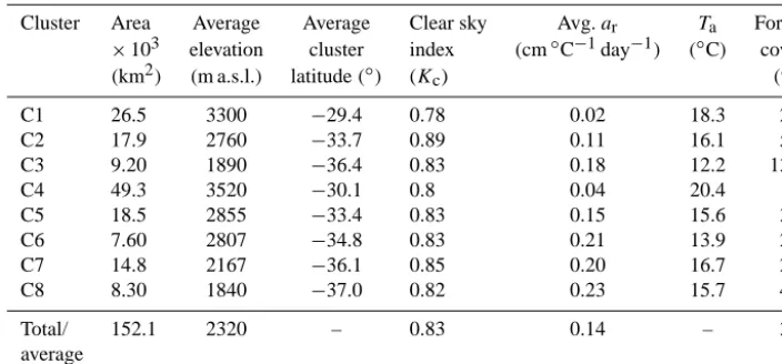
Table 1. Study area subdivision, relevant characteristics and model parameters.

Cluster Area Average Average Clear sky Avg.ar Ta Forest ×103 elevation cluster index (cm◦C−1day−1) (◦C) cover

(km2) (m a.s.l.) latitude(◦) (Kc) (%)

C1 26.5 3300 −29.4 0.78 0.02 18.3 2.0 C2 17.9 2760 −33.7 0.89 0.11 16.1 5.5 C3 9.20 1890 −36.4 0.83 0.18 12.2 13.8 C4 49.3 3520 −30.1 0.8 0.04 20.4 1.4 C5 18.5 2855 −33.4 0.83 0.15 15.6 3.0 C6 7.60 2807 −34.8 0.83 0.21 13.9 2.3 C7 14.8 2167 −36.1 0.85 0.20 16.7 2.5 C8 8.30 1840 −37.0 0.82 0.23 15.7 4.9

Total/ 152.1 2320 – 0.83 0.14 – 3.3 average

Table 2. Snow-pillow measurements available within the study domain.

ID SWE data Symbol Lat. Long. Elevation Reference (S) (W) (m a.s.l.) cluster

Chile

1 Quebrada Larga QUE 30◦430 70◦160 3500 C1 2 Cerro Vega Negra CVN 30◦540 70◦300 3600 C1 3 El Soldado SOL 32◦000 70◦190 3290 C2 4 Portillo POR 32◦500 70◦060 3000 C2 5 Laguna Negra LAG 33◦390 70◦060 2780 C2 6 Lo Aguirre LOA 35◦580 70◦340 2000 C3 7 Alto Mallines ALT 37◦090 70◦140 1770 C3

Argentina

8 Toscas TOS 33◦090 69◦530 3000 C5 9 Laguna Diamante DIA 34◦110 69◦410 3300 C6 10 Laguna Atuel ATU 34◦300 70◦020 3420 C6 11 Valle Hermoso VAL 35◦080 70◦120 2250 C7 12 Paso Pehuenches PEH 35◦080 70◦230 2545 C7

(cm◦_C−1_day−1_{), which is similar to values reported in} pre-vious studies performed in other mountain ranges in the Northern Hemisphere (0.20–0.25 in Martinec, 1989; 0.17 in Kustas et al., 1994; 0.20 in Brubaker at al., 1996; 0.15 in Molotch and Margulis, 2008). However, values associated with the northernmost clusters of our study area are quite low, reaching under 0.02 for the C1 cluster in northern Chile. Clear sky index (Kc) values range between 0.78 and 0.89, which is similar to values reported by Salazar and Raichijk (2014), who estimateKcvalues on the order of 0.90 for a single location at 1200 m a.s.l. in northern Argentina. A 5 to 6◦C difference can be observed in mean air tempera-ture at index stations between the northern and southern edge of the domain. Temperatures for the C4 cluster are subject to greater uncertainty, because no high-elevation climate station data were available for this study (Fig. S4). Forest cover val-ues are lower than 6 % throughout the model domain, with

the exception of cluster C3, with a value of 13.8 %. The dif-ference in forest cover between clusters C3 and C8 can be attributed to the precipitation shadow effect induced by the Andes ridge. Forest corrections applied to MODIS fSCA re-sulted in a 17 % increase with respect to the original values over the southern sub-domain (C3).

3.4 Evaluation data: SWE, snow depth and river flow observations

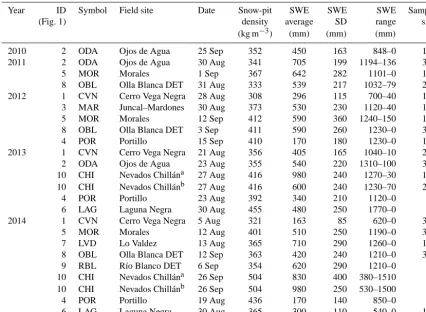
er-Table 3. Summary of snow depth and density intensive study campaigns.

Year ID Symbol Field site Date Snow-pit SWE SWE SWE Sample (Fig. 1) density average SD range size

(kg m−3) (mm) (mm) (mm)

2010 2 ODA Ojos de Agua 25 Sep 352 450 163 848–0 134 2011 2 ODA Ojos de Agua 30 Aug 341 705 199 1194–136 374 5 MOR Morales 1 Sep 367 642 282 1101–0 171 8 OBL Olla Blanca DET 31 Aug 333 539 217 1032–79 289 2012 1 CVN Cerro Vega Negra 28 Aug 308 296 115 700–40 166 3 MAR Juncal–Mardones 30 Aug 373 530 230 1120–40 163 5 MOR Morales 12 Sep 412 590 360 1240–150 152 8 OBL Olla Blanca DET 3 Sep 411 590 260 1230–0 309 4 POR Portillo 15 Sep 410 170 180 1230–0 181 2013 1 CVN Cerro Vega Negra 21 Aug 356 405 165 1040–10 282 2 ODA Ojos de Agua 23 Aug 355 540 220 1310–100 300 10 CHI Nevados Chillána 27 Aug 416 980 240 1270–30 104 10 CHI Nevados Chillánb 27 Aug 416 600 240 1230–70 216 4 POR Portillo 23 Aug 392 340 210 1120–0 91 6 LAG Laguna Negra 30 Aug 455 480 250 1770–0 32 2014 1 CVN Cerro Vega Negra 5 Aug 321 163 85 620–0 326 5 MOR Morales 12 Aug 401 510 250 1190–0 329 7 LVD Lo Valdez 13 Aug 365 710 290 1260–0 186 8 OBL Olla Blanca DET 12 Sep 363 420 240 1210–0 334 9 RBL Río Blanco DET 6 Sep 354 620 290 1210–0 99 10 CHI Nevados Chillána 26 Sep 504 830 400 380–1510 18 10 CHI Nevados Chillánb 26 Sep 504 980 250 530–1500 87 4 POR Portillo 19 Aug 436 170 140 850–0 73 6 LAG Laguna Negra 30 Aug 365 300 110 540–0 117

a_{Without forest cover (upper part of basin).}b_{With forest cover (lower part of basin).}

rors and data gaps. An analysis of the seasonal variability of snow-pillow records on the western and eastern slopes of the Andes suggests that the peak-SWE date is somewhat de-layed on the latter, by approximately 1 month. Therefore, peak-SWE estimates for Chilean and Argentinean stations are evaluated on 1 September and 1 October, respectively, although in the results section we show values for 15 Septem-ber in order to use a unique date for the entire domain. Man-ual snow depth observations were taken in the vicinity of selected snow-pillow locations in order to evaluate the rep-resentativeness of these measurements at the MODIS grid scale during the peak-SWE time window. These depth obser-vations were obtained in regular grid patterns within an area the approximate size of a MODIS pixel (500 m), centered about the snow-pillow location. On average, 120 depth obser-vations spaced at approximately 50 m increments were ob-tained at each snow-pillow site. Snow density was estimated by a depth-weighted average of snow densities measured in snow pits with a 1000-cc snow cutter. Samples where ob-tained either at regular 10 cm depth intervals along the snow pit face, or at the approximate mid depth of identifiable snow strata for very shallow snow pack conditions. Weights were computed as the fraction of total depth represented by each snow sample.

Distributed snow depth observations were available from snow surveys carried out during late winter between 2010 and 2014 at seven study catchments on the western side of the Andes, between latitudes 30 and 37◦_{S (Fig. 1, Table 3).}

Spring and summer season (September to March) total river flow volume (SSRV) for the 2001–2014 period is ob-tained from unimpaired (no human extractions) streamflow records at river gauges located in the mountain front along the model domain. Data were pre-selected leaving out series that showed too many missing values, and verified through the double mass curve method (Searcy and Hardison, 1960) in order to discard anomalous values and to ensure ho-mogeneity throughout the period of study. Regional con-sistency was verified through regression analysis, only in-cluding streamflow records withR2 values greater than 0.5 among neighboring catchments. Missing values constituted about 3.7 % of the entire period and were filled through lin-ear regression.

4 Results

4.1 Model validation

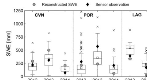
Figure 3 compares reconstructed peak SWE (gray circles) to observed values at three snow-pillow locations (black dia-monds) where additional validation sampling at the MODIS pixel scale was conducted (box plots). At the Cerro Vega Ne-gra site (CVN), located in cluster C1, the model overesti-mates peak SWE (1 September) with respect to the snow-pillow value by 97 % in 2013 and by 198 % in 2014. At the Portillo site (POR, cluster C2), reconstructed SWE underes-timates recorded values by 51 % in 2013 and 72 % in 2014. At the Laguna Negra site (LAG, also C2), reconstructed peak SWE slightly overestimates recorded values (8 %) (Ta-ble 4). However, reconstructed SWE compares favorably to distributed manual SWE observations obtained in the vicin-ity of the snow pillows at the POR and LAG sites. At POR, model estimates approach upper (2012) and lower (2013 and 2104) quartiles, while at LAG the model estimates are closer to the minimum value observed in 2013 and very similar to the observed mean in 2014.

Figure 4 depicts the comparison between reconstructed SWE and snow surveys carried out at pilot basins throughout the model domain. From left to right, it can be seen that the model slightly overestimates SWE with respect to observa-tions at CVN (i.e., 18 % overestimation). Further south, there is a very good agreement at ODA-MAR (i.e., 4 % underesti-mation), with less favorable results at MOR-LVD (i.e., 39 % underestimation) and OB-RBL (i.e., 36 % underestimation). At CHI the model significantly underestimates SWE (i.e., by 67 %); note that this site is heavily forested. For the 2013a and 2014a boxes (Fig. 4) – which correspond to clearing sites – there is still underestimation, but of lesser magnitude (20 %). Summarizing, we detect model overestimation with respect to snow survey medians in four cases and underesti-mation in fifteen cases. In 11 out of 19 cases, reconstructed SWE lies within the snow survey data uncertainty bounds (standard deviation).

Figure 3. Reconstructed SWE validation at selected snow-pillow

sites. Black diamonds are instrumental records, gray circles are model estimates, and box plots summarize the manual verification data set around the pillow site. Upper and lower box limits are the 75 and 25 % quartiles, the horizontal line is the median, the white box is the mean, upper and lower dashes represent plus and minus 2.5 SD from the mean, and crosses are outlying values.

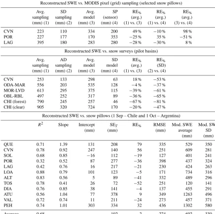
Table 4. Model validation statistics against intensive study area observations around snow pillows and at catchment scale.

Reconstructed SWE vs. MODIS pixel (grid) sampling (selected snow pillows)

Avg. SD Avg. SP RE% RE% RE% sampling sampling model (sensor) (avg.) (avg.) (avg.) (mm)(1) (mm)(2) (mm)(3) (mm)(4) (1) vs. (3) (1) vs. (4) (3) vs. (4)

CVN 223 110 334 200 49 % −10 % 98 % POR 227 177 170 353 −25 % 35 % −51 % LAG 395 180 283 280 −28 % −30 % 8 %

Reconstructed SWE vs. snow surveys (pilot basins)

Avg. AD Avg. SD RE% RE% sampling sampling model model (avg.) (SD) (mm)(1) (mm)(2) (mm)(3) (mm)(4) (1) vs. (3) (2) vs. (4)

CVN 253 133 298 63 18 % −53 % ODA-MAR 556 203 535 128 −4 % −37 % MOR-LVD 613 295 375 115 −39 % −61 % OBL-RBL 497 252 317 89 −36 % −65 % CHI (forest) 790 245 257 46 −67 % −81 % CHI (clear) 905 320 724 170 −20 % −47 %

Reconstructed SWE vs. snow pillows (1 Sep – Chile and 1 Oct – Argentina)

R2 Slope Intercept SEx RE% RMSE Mod. SWE Mod. SWE (mm) (mm) (mm) average SD

(mm) (mm)

QUE 0.71 1.39 131 208 79 335 529 350 CVN 0.78 0.92 247 140 56 251 609 281 SOL 0.68 0.85 −16 112 −19 127 401 241 POR 0.32 0.52 87 277 −36 398 437 324 LAG 0.42 0.76 16 217 −21 230 424 263 LOA 0.88 0.79 101 123 −5 171 734 316

ALT 0.83 0.56 5 89 −41 332 489 296

TOS 0.78 0.41 26 72 −52 251 120 141 DIA 0.76 0.85 38 141 −4 137 455 291

ATU 0.56 1.04 77 378 9 349 1263 496

VAL 0.72 0.74 11 211 −24 273 457 371 PEH 0.74 1.01 303 334 32 436 1302 580

Average 0.68 – – 192 −2 274 602 330

Figure 4. Reconstructed SWE validation at pixels with snow survey data. Box plots summarize all individual measurements at pixels

Figure 5. Comparison between peak reconstructed and observed

SWE at snow-pillow sites. Solid line represents the 1 : 1 line.

pillows, the model estimates are lower than the sensor ob-servation; the range of relative errors for those sites with un-derestimation goes from−52 to−5 %.

4.2 Correlation with melt-season river flows

Under the assumption of unimpaired flows, peak SWE and seasonal flow volume should show some degree of correla-tion, even though no assumptions can be made here about other relevant hydrologic processes, such as flow contribu-tions from glaciated areas, subsurface storage carryover at the basin scale and influence of spring and summer precip-itation. Differences can be expected due to losses to evap-otranspiration and sublimation affecting the snowpack and soil water throughout the melt season. Hence, basin-averaged peak SWE should always be higher than melt season river volume. A clear regional pattern emerges when inspecting the results of this comparison in Fig. 6. Correlation between peak SWE and melt season river flow is higher in clusters C1 and C4 withR2values of 0.84 and 0.86, respectively. The

re-Figure 6. Area-specific spring–summer runoff volume (SSRV)

ver-sus peak SWE. Clusters 1 through 3 include rivers on the Chilean (western) slope of the Andes range; clusters 4 through 8 correspond to Argentinean (eastern) rivers. Solid line represents the 1 : 1 line. C4 and C8 SSRV were estimated by the area-transpose method.

Table 5. Coefficient of determinationR2between river melt season flows (SSRV) and estimated and observed SWE (end-of-winter). R2value-specific SSRV vs. R2value-specific SSRV vs.

estimated SWE per cluster SWE at snow pillows (2001–2013)∗

2001–2014 Neglecting 2009 Best Second best at Argentinean

clusters∗∗

C1 0.84 – 0.74 (CVN) 0.69 (QUE) C2 0.78 – 0.82 (LAG) 0.68 (POR) C3 0.57 – 0.17 (LOA) 0.16 (ALT)

C4 0.87 – – –

C5 0.66 0.82 0.81 (TOS) – C6 0.45 0.76 0.87 (ATU) 0.77 (DIA) C7 0.64 0.89 0.77 (VAL) 0.41 (PEH)

C8 0.48 0.64 – –

∗_{2014 flows in Argentina unavailable to us at the time of writing.}∗∗_{2009 is considered an outlier year for}

the reconstruction at Argentinean sites.

(POR, with a value of 0.68). For the eastern side of the conti-nental divide, the distributed product shows similar skill than that of snow pillows except for Atuel, which has a very high correlation (R2of 0.87) with cluster C6 river flows, and for cluster C7, in which the reconstruction shows higher predic-tive power (R2of 0.89) than the available SWE observations (VAL and PEH).

4.3 Regional SWE estimates

Figure 7 shows the 15 September SWE average over the 2001–2014 period obtained from the reconstruction model, and the percent annual deviations (anomalies) from that av-erage. Steep elevation gradients can be inferred from the cli-matology, as well as the latitudinal variation expected from precipitation spatial patterns. For the northern clusters (C1 and C4), the peak SWE averaged over snow-covered areas is on the order of 300 mm, while in the middle of the domain (C2, C5, C6), it averages approximately 750 mm. The south-ern clusters (C3, C7, C8) do show high accumulation aver-ages (≈650 mm), despite the sharp decrease in the Andes elevation south of latitude 34◦S. The anomaly maps convey the important degree of inter-annual variability, as well as distinct spatial patterns associated with it. Between 2001 and 2014, years 2002 and 2005 stand out for displaying large pos-itive anomalies throughout the entire mountainous region of the model domain, with values 2000 mm and more above the simulation period average. Other years prior to 2010 show differential accumulation patterns, where either the northern or southern parts of the domain are more strongly affected by positive or negative anomalies. Overall, the northern clus-ters (C1 and C4) show above-average accumulation in only 3 (2002, 2005 and 2007) of the 14 simulated years, whereas the other clusters show above-average accumulation for 6 years (2001, 2002, 2005, 2006, 2008 and 2009). In particular, years 2007 and 2009 show a bimodal spatial structure, with excess

accumulation (deficit) in the northern (southern) clusters dur-ing the former, and the inverse pattern in the latter year.

A longitudinal pattern in the distribution of negative anomalies can be discerned from Fig. 7, whereby drought conditions tend to be more acute on one side of the divide versus the other. Conversely, during positive anomaly years, both sides of the Andes seem to show similar behavior. Fur-ther research on the mechanisms of moisture transport during below-average precipitation years may shed light on this re-sult.

SWE-Figure 7. Regional peak (15 September) SWE climatology for the 2001–2014 period (upper left panel), and annual peak SWE anomalies.

elevation distribution in C6 and C7 when compared to C3. On the eastern side of the model domain, it is interesting to see a steepening of the average peak SWE elevation profile between C6 and C8, suggesting that C8 is less affected by Andes blockage than its northern counterparts.

Estimated net energy inputs (Fig. 9) shows a decrease from the northern (C1 and C4) into the mid-range clusters (C2, C5 and C6), with increases again in the southern reaches of the domain (C3, C7 and C8). This is a result of a combination of an increasing trend in net shortwave radiation in the south– north direction and a reverse spatial trend in net longwave radiation exchange, which increases (approaches less nega-tive values) in the north–south direction. Modeled turbulent energy fluxes (Eq. 1) are negligible in the northern clusters, but their contribution to the net energy exchange increases with latitude as a result of the spatial variation in thear pa-rameter.

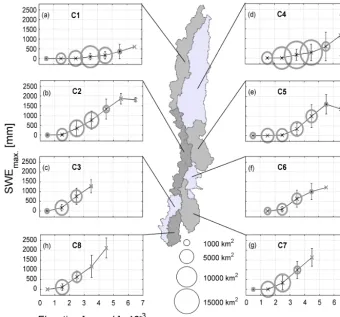
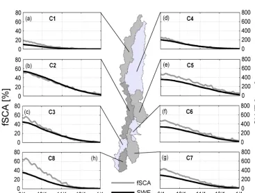
Figure 10 shows the temporal (seasonal) variation in av-erage fSCA and SWE for each cluster, and Table 6 shows peak SWE at the watershed scale, averaged both over the en-tire basin and over the snow-covered area. Maximum fSCA increases in the north–south direction, consistent with the cli-matological increase in winter precipitation and decrease in

Figure 8. Maximum SWE through 1000 m elevation bands (EB). Crosses are mean values within EB, lines are the estimated SWE-elevation

profile. Circle radius indicates EB area (km2) scaled by 0.05 and takes values from the SWE axis.

domain, but peak SWE is not significantly higher than the estimates in the other clusters on the Argentinean side of the Andes.

5 Discussion

5.1 Sensitivity analysis

The Andes Cordillera, on the one hand, displays ideal con-ditions for SWE reconstruction, including low cloud cover, infrequent snowfall during spring and summer, and very low forest cover. On the other hand, the scarcity of basic climate data poses challenges that would affect any modeling exer-cise. A local sensitivity analysis is implemented in order to gain insights regarding the influence of some of the assump-tions required for SWE modeling (Fig. 11). The influence of the clear sky factor (Kc), snow surface albedo (∝s), the slope of the 1LST vs.1Ta relationship (µ), thear parameter, and

the difference between air and snow surface temperature are explored. Results are shown for the model pixels correspond-ing to two of the snow-pillow sites, each located at the north-ern and southnorth-ern sub-regions of the model domain respec-tively. The clear sky factor, snow albedo and 1LSTvs.1Ta

slope are the most sensitive parameters at the northern (CVN) site. Increasing the slope in the1LST vs.1Ta relationship

There-Figure 9. Time series of energy fluxes over snow surface (average over 14 years) and global average per cluster. Unique axes scale for all

plots.

Figure 10. Average seasonal evolution of fSCA and SWE in the study region. Lower right panel shows the spatial correlation between

Table 6. Peak SWE 2001–2014 climatology for river basins within the study region. Basin-wide averages, SCA-wide averages and

basin-wide water volumes shown.

ID Basin – gauge station Lat. S Long. W Outlet Area SWE

elev. (km2) Basin-wide Over SCA Basin-wide (m a.s.l.) (mm) (mm) (m3×10−6)

Chile

1 Copiapó en Pastillo 27◦590 69◦580 1300 7470 45 120 336 2 Huasco en Algodones 28◦430 70◦300 750 7180 68 161 488 3 Elqui en Algarrobal 29◦590 70◦350 760 5710 151 269 862 4 Hurtado en San Agustín 30◦270 70◦320 2050 676 302 325 204 5 Grande en Puntilla San Juan 30◦410 70◦550 2140 3545 137 306 486 6 Cogotí en La Fraguita 31◦060 70◦530 1021 491 182 335 89 7 Illapel en Huintil 31◦330 70◦570 650 1046 180 305 188 8 Chalinga en San Agustín 31◦410 70◦430 920 437 142 332 62 9 Choapa en Salamanca 31◦480 70◦550 560 2212 214 356 473 10 Sobrante en Piñadero 32◦120 70◦420 2057 126 172 198 22 11 Alicahue en Colliguay 32◦180 70◦440 852 344 92 184 32 12 Putaendo en Resg. Los Patos 32◦300 70◦340 1218 890 273 346 243 13 Aconcagua en Chacabuquito 32◦510 70◦300 950 2110 609 692 1285 14 Mapocho en Los Almendros 33◦220 70◦270 970 640 269 342 172 15 Maipo en El Manzano 33◦350 70◦220 850 4840 692 760 3349 16 Cachapoal en Puente Termas 34◦150 70◦340 700 2455 700 814 1719 17 Tinguiririca en Los Briones 34◦430 70◦490 560 1785 532 677 950 18 Teno en Claro 34◦590 70◦490 650 1210 438 524 530 19 Lontué en Colorado–Palos 35◦150 71◦020 600 1330 656 759 872 20 Maule en Armerillo 35◦420 70◦100 470 5465 525 554 2869 21 Ñuble en San Fabián 36◦340 71◦330 410 1660 376 430 624 22 Polcura en Laja 37◦190 77◦320 675 2088 358 378 748

Argentina

23 Jachal en Pachimoco 30◦120 68◦490 1563 24 266 79 175 1917 24 San Juan en km 101 31◦150 69◦100 1129 23 860 308 569 7349 25 Mendoza en Guido 32◦540 69◦140 1479 7304 460 672 3360 26 Tunuyán en Zapata 33◦460 69◦160 852 11 230 289 592 3245 27 Diamante en La Jaula 34◦400 69◦180 1451 2832 395 489 1118 28 Atuel en Loma Negra 35◦150 69◦140 1353 3696 338 525 1249 39 Malargue en La Barda 35◦330 69◦400 1568 1055 171 284 180 30 Colorado en Buta Ranquil 37◦040 69◦440 817 14 896 288 495 4290 31 Neuquén en Rahueco 37◦210 70◦270 870 8266 356 446 2943

fore, perturbations of the other terms account for a smaller fraction of the energy exchange at the southern sites. 5.2 Model performance and conceptual energy balance

representation

Among the many factors that influence model performance, the sub-region delineation involves the selection of index meteorological stations for extrapolating input data at the domain level. Thus, for example, two adjacent pixels that are part of different sub-regions may be assigned input data derived from two different meteorological stations that are many kilometers apart. It would be preferable to use dis-tributed inputs only, but these were not available for this

do-main. Future research is needed to explore alternative strate-gies for domain clustering.

Figure 11. Sensitivity of peak SWE estimates to model forcings and

parameters. Average over the 2001–2014 period at selected snow-pillow sites.1xrepresents the percentage change over each param-eter studied with respect to the base case.

this value is strongly affected by two stations where we ob-served significant overestimation (QUE and CVN). When including the remaining ten snow pillows only, relative er-ror increases to −16 %. Given that forest cover is mini-mal in our modeling domain, we can attribute this bias to either weaknesses in the simplified energy balance model formulation or to errors in the MOD10A1 fSCA product. Previous work in the northern hemisphere (Rittger et al., 2013) has shown that MODIS can underestimate fractional snow cover during the snowmelt season. On the one hand, land cover heterogeneity at spatial resolutions lower than the MODIS scale (i.e., 500 m) results in mixed-pixel detec-tion problems. On the other hand, spectral unmixing based on the NDSI approach tends to underestimate fSCA un-der patchy snow distributions. In addition, surface temper-atures greater than 10◦C – more likely to exist during late spring – induce MODIS fSCA underestimation. Molotch and Margulis (2008) tested the SWE reconstruction model us-ing Landsat ETM and MOD10A1 and found that maximum basin-wide mean SWE estimates were significantly lower when using MOD10A1. More recently, Cortés et al. (2014a) showed that a similar pattern can be seen for the extratrop-ical Andes, whereby MODIS fSCA consistently underesti-mated LANDSAT TM fSCA retrievals. MODIS fSCA under-estimation during spring combined with increased net energy fluxes over the snowpack can result in a marked underestima-tion (∼20 %) for available energy flux for snowpack melting and consequently (∼45 %) for maximum SWE (Molotch and Margulis, 2008).

Figure 12. Restricted degree-day factor as a function of space

(basin cluster) and climatological properties. Bowen (β) coefficient shown between parentheses in the legend.

Comparisons against spatial interpolations from intensive-study areas in the Sierra Nevada or Rocky Mountains (e.g., Erxleben et al., 2002; Jepsen et al., 2012) are not di-rectly applicable, because in this study we do not employ in-terpolation methods to derive our manual snow survey SWE estimates. However, the average overestimation found with respect to snow survey data could be explained by the fact that manual surveys are limited by site accessibility and sam-pling procedures. For example, snow probes utilized are only 3.0 m long, which precludes observation of deeper snow-pack; likewise, deep snow is expected in sites exposed to avalanching, which were generally avoided in snow survey design due to safety considerations. On the other hand, man-ual snow surveys do not visit steep snow-free areas where snow depth is expected to be lower than the 500 m pixel re-construction. The combined effect of these two contrasting effects is the subject of further research in this region.

although pseudo-physically based – compared to degree-day or fully calibrated models – allows only for positive net tur-bulent fluxes, because both thearand the degree-day temper-ature index are positive values. However, previous studies in this region (Corripio and Purves, 2005; Favier et al., 2009) have suggested that latent heat fluxes have a relevant role be-cause of high sublimation rates favored by high winds and low relative humidity conditions predominant in the area.

In order to diagnose differential performance of the model across the hydrologic units defined in this study, we com-pute the Bowen ratio (β) at the point scale from data avail-able only at the few high-elevation meteorological stations in the region with recorded relative humidity. The calculations show that at stations located within cluster C1, latent heat fluxes are opposite in sign and larger in magnitude than sen-sible heat fluxes (Fig. S6). While this results in net turbulent cooling of the snowpack, this energy loss is not considered in our simplified energy balance approach. Note that for the clusters C5, C6, C7 and C8, all located on the eastern (Ar-gentinean) slope of the Andes, sensible and latent heat fluxes are positive, compared to negative latent heat fluxes for all the index stations within clusters C2 and C3 on the Chilean side. This result is consistent with Insel et al. (2010), who ap-plied a regional circulation model (RegCM3) in the area and showed a significant difference in relative humidity (∼70 % on the eastern side vs.∼40 % on the western side). The fact that we extrapolate the ar parameter value based on rela-tively low elevation meteorological observations throughout the southern Argentinean hydrologic units may result in a yet not quantified overestimation of seasonal energy inputs and peak SWE for those clusters.

6 Conclusions

Snow water equivalent is the foremost water source for the extratropical Andes region in South America. This paper presents the first high-resolution distributed assessment of this critical resource, combining instrumental records with remotely sensed snow-covered area and a physically based snow energy balance model. Overall errors in estimated peak SWE, when compared with operational station data, amount to−2.2 %, and correlation with observed melt-season river flows is high, with an R2 value of 0.80. MODIS fractional SCA data proved adequate for the goals of this study, afford-ing high temporal resolution observations and an appropriate spatial resolution given the extent of the study region. These results have implications for evaluating seasonal water sup-ply forecasts, analyzing synoptic-scale drivers of snow ac-cumulation, and validating precipitation estimates from re-gional climate models. In addition, the strong correlation between peak SWE and seasonal river flow indicates that our results could be useful for the evaluation of alternative water resource projects as part of development and climate change adaptation initiatives. Finally, the regional SWE and

anomaly estimates illustrate the dramatic spatial and tempo-ral variability of water resources in the extratropical Andes, and provide a striking visual assessment of the progression of the drought that has affected the region since 2009. These results should motivate further research looking into the cli-matic drivers of this spatially distributed phenomenon.

The Supplement related to this article is available online at doi:10.5194/hess-20-411-2016-supplement.

Acknowledgements. This research was conducted with support from CONICYT, under grants FONDECYT 1121184, SER-03, FONDEF CA13I10277 and CHILE-USA2013. The authors wish to thank everybody involved in field data collection, including brothers Santiago and Gonzalo Montserrat, Mauricio Cartes, Alvaro Ayala, and many others. Gonzalo Cortés provided insightful comments to working drafts of this paper.

Edited by: C. De Michele

References

Aceituno, P.: On the functioning of the Southern Oscillation in the South American sector. Part I: Surface climate, Mon. Weather Rev., 116, 505–524, 1988.

Ahl, D. E., Gower, S. T., Burrows, S. N., Shabanov, N. V., Myneni, R. B., and Knyazikhin, Y.: Monitoring spring canopy phenology of a deciduous broadleaf forest using MODIS, Remote Sens. En-viron., 104, 88–95, 2006.

Aravena, J.-C. and Luckman, B. H.: Spatio-temporal rainfall pat-terns in southern South America, Int. J. Climatol., 29, 2106– 2120, 2009.

Army Corps of Engineers: Engineering and design: runoff from snowmelt, Washington, 1960.

Arsenault, K. R., Houser, P. R., and De Lannoy, G. J. M.: Evaluation of the MODIS snow cover fraction product, Hydrol. Process., 28, 980–998, doi:10.1002/hyp.9636, 2014.

Ayala, A., McPhee, J., and Vargas, X.: Altitudinal gradients, mid-winter melt, and wind effects on snow accumulation in semiarid midlatitude Andes under La Niña conditions, Water Resour. Res., 50, 3589–3594, doi:10.1002/2013WR014960, 2014.

Benali, A., Carvalho, A. C., Nunes, J. P., Carvalhais, N., and Santos, A.: Estimating air surface temperature in Portugal using MODIS LST data, Remote Sens. Environ., 124, 108–121, 2012. Brubaker, K., Rango, A., and Kustas, W.: Incorporating

Ra-diation Inputs into the Snowmelt Runoff Model, Hy-drol. Process., 10, 1329–1343, doi:10.1002/(SICI)1099-1085(199610)10:10<1329::AID-HYP464>3.0.CO;2-W, 1996. Castro, L. M., Gironás, J., and Fernández, B.: Spatial estimation of

daily precipitation in regions with complex relief and scarce data using terrain orientation, J. Hydrol., 517, 481–492, 2014. Cline, D. W., Bales, R. C., and Dozier, J.: Estimating the spatial

Colombi, A., De Michele, C., Pepe, M., and Rampini, A.: Estima-tion of daily mean air temperature from MODIS LST in Alpine areas, EARSeL EProceedings 6, 38–46, 2007.

Corripio, J. G. and Purves, R. S.:. Surface energy balance of high altitude glaciers in the central Andes: The effect of snow pen-itentes, in: Clim. Hydrol. Mt. Areas, edited by: Collins, D., de Jong, C., and Ranzi, R., Wiley, London, 15–27, 2005.

Cortés, G., Vargas, X., and McPhee, J.: Climatic sensitivity of streamflow timing in the extratropical western Andes Cordillera, J. Hydrol., 405, 93–109, doi:10.1016/j.jhydrol.2011.05.013, 2011.

Cortés, G., Cornwell, E., McPhee, J. P., and Margulis, S. A.: Snow Cover Quantification in the Central Andes Derived from Multi-Sensor Data, in: AGU Fall Meeting Abstracts, San Francisco, p. 0410, 2014a.

Cortés, G., Girotto, M., and Margulis, S. A.: Analysis of sub-pixel snow and ice extent over the extratropical Andes using spectral unmixing of historical Landsat imagery, Remote Sens. Environ., 141, 64–78, doi:10.1016/j.rse.2013.10.023, 2014b.

DeWalle, D. and Rango, A.: Principles of snow hydrology, Cam-bridge University Press, New York, 2008.

Dietz, A. J., Kuenzer, C., Gessner, U., and Dech, S.: Remote sensing of snow – a review of available methods, Int. J. Remote Sens., 33, 4094–4134, 2012.

Erxleben, J., Elder, K., and Davis, R.: Comparison of spatial in-terpolation methods for estimating snow distribution in the Col-orado Rocky Mountains, Hydrol. Process., 16, 3627–3649, 2002. Eva, H. D., Belward, A. S., De Miranda, E. E., Di Bella, C. M., Gond, V., Huber, O., Jones, S., Sgrenzaroli, M., and Fritz, S.: A land cover map of South America, Global Change Biol., 10, 731–744, 2004.

Falvey, M. and Garreaud, R.: Wintertime precipitation episodes in central Chile: Associated meteorological conditions and oro-graphic influences, J. Hydrometeorol., 8, 171–193, 2007. Falvey, M. and Garreaud, R. D.: Regional cooling in a

warm-ing world: Recent temperature trends in the southeast Pa-cific and along the west coast of subtropical South Amer-ica (1979–2006), J. Geophys. Res.-Atmos., 114, D04102, doi:10.1029/2008JD010519, 2009.

Favier, V., Falvey, M., Rabatel, A., Praderio, E., and López, D.: Interpreting discrepancies between discharge and precipitation in high-altitude area of Chile’s Norte Chico region (26–32◦S). Water Resour. Res., 45, W02424, doi:10.1029/2008WR006802, 2009.

Gafurov, A. and Bárdossy, A.: Cloud removal methodology from MODIS snow cover product, Hydrol. Earth Syst. Sci., 13, 1361– 1373, doi:10.5194/hess-13-1361-2009, 2009.

Garreaud, R. D.: The Andes climate and weather, Adv. Geosci., 22, 3–11, doi:10.5194/adgeo-22-3-2009, 2009.

Gascoin, S., Lhermitte, S., Kinnard, C., Bortels, K., and Liston, G. E.: Wind effects on snow cover in Pascua-Lama, Dry Andes of Chile, Adv. Water Resour., 55, 25–39, doi:10.1016/j.advwatres.2012.11.013, 2013.

Guan, B., Molotch, N. P., Waliser, D. E., Jepsen, S. M., Painter, T. H., and Dozier, J.: Snow water equivalent in the Sierra Nevada: Blending snow sensor observations with snowmelt model simulations, Water Resour. Res., 49, 5029– 5046, doi:10.1002/wrcr.20387, 2013.

Hall, D. K. and Riggs, G. A.: Accuracy assessment of the MODIS snow products, Hydrol. Process., 21, 1534–1547, 2007. Hall, D. K., Riggs, G. A., Salomonson, V. V., DiGirolamo, N. E.,

and Bayr, K. J.: MODIS snow-cover products, Remote Sens. En-viron., 83, 181–194, 2002.

Hansen, M. C., DeFries, R. S., Townshend, J. R. G., Carroll, M., Dimiceli, C., and Sohlberg, R. A.: Global percent tree cover at a spatial resolution of 500 meters: First results of the MODIS vegetation continuous fields algorithm, Earth Interact., 7, 1–15, 2003.

Hofierka, J. and Suri, M.: The solar radiation model for Open source GIS: implementation and applications, in: Proceedings of the Open Source GIS-GRASS Users Conference, Trento, Italy, 1– 19, 2002.

Huete, A., Didan, K., Miura, T., Rodriguez, E. P., Gao, X., and Fer-reira, L. G.: Overview of the radiometric and biophysical perfor-mance of the MODIS vegetation indices, Remote Sens. Environ., 83, 195–213, 2002.

Insel, N., Poulsen, C. J., and Ehlers, T. A.: Influence of the Andes Mountains on South American moisture transport, convection, and precipitation, Clim. Dynam., 35, 1477–1492, 2010. Jepsen, S. M., Molotch, N. P., Williams, M. W., Rittger, K. E.,

and Sickman, J. O.: Interannual variability of snowmelt in the Sierra Nevada and Rocky Mountains, United States: Examples from two alpine watersheds, Water Resour. Res., 48, W02529, doi:10.1029/2011WR011006, 2012.

Krogh, S. A., Pomeroy, J. W., and McPhee, J.: Physically Based Mountain Hydrological Modeling Using Reanalysis Data in Patagonia, J. Hydrometeorol., 16, 172–193, doi:10.1175/JHM-D-13-0178.1, 2015.

Kustas, W. P., Rango, A., and Uijlenhoet, R.: A simple energy bud-get algorithm for the snowmelt runoff model.,Water Resour. Res., 30, 1515–1527, 1994.

Martinec, J.: Hour-to-hour snowmelt rates and lysimeter outflow during an entire ablation period, Snow Cover Glacier Var., in: Glacier and Snow Cover Variations, IAHS Publ. no. 183, edited by: Colbeck, S. C., Proceedings of the Baltimore Symposium, Maryland, 19–28, 1989.

Masiokas, M. H., Villalba, R., Luckman, B. H., Le Quesne, C., and Aravena, J. C.: Snowpack variations in the central Andes of Argentina and Chile, 1951–2005: Large-scale atmospheric in-fluences and implications for water resources in the region, J. Climate, 19, 6334–6352, 2006.

Meromy, L., Molotch, N. P., Link, T. E., Fassnacht, S. R., and Rice, R.: Subgrid variability of snow water equivalent at operational snow stations in the western USA, Hydrol. Process., 27, 2383– 2400, 2013.

Minder, J. R., Mote, P. W., and Lundquist, J. D.: Surface tempera-ture lapse rates over complex terrain: Lessons from the Cascade Mountains, J. Geophys. Res.-Atmos., 115, 1984–2012, 2010. Molotch, N. P.: Reconstructing snow water equivalent in the Rio

Grande headwaters using remotely sensed snow cover data and a spatially distributed snowmelt model, Hydrol. Process., 23, 1076–1089, doi:10.1002/hyp.7206, 2009.

Molotch, N. P. and Margulis, S. A.: Estimating the distribution of snow water equivalent using remotely sensed snow cover data and a spatially distributed snowmelt model: A multi-resolution, multi-sensor comparison, Adv. Water Resour., 31, 1503–1514, doi:10.1016/j.advwatres.2008.07.017, 2008.

Montgomery, D. R., Balco, G., and Willett, S. D.: Climate, tecton-ics, and the morphology of the Andes, Geology, 29, 579–582, 2001.

Neteler, M.: Estimating Daily Land Surface Temperatures in Moun-tainous Environments by Reconstructed MODIS LST Data, Re-mote Sens., 2, 333–351, doi:10.3390/rs1020333, 2010.

Neteler, M., Bowman, M. H., Landa, M., and Metz, M.: GRASS GIS: A multi-purpose open source GIS, Environ. Model. Softw., 31, 124–130, 2012.

Newman, M., Compo, G. P., and Alexander, M. A.: ENSO-forced variability of the Pacific decadal oscillation, J. Climate, 16, 3853–3857, 2003.

Núñez, J., Rivera, D., Oyarzún, R., and Arumí, J. L.: Influence of Pacific Ocean multidecadal variability on the distributional prop-erties of hydrological variables in north-central Chile, J. Hydrol., 501, 227–240, 2013.

Pomeroy, J. W., Marks, D., Link, T., Ellis, C., Hardy, J., Rowlands, A., and Granger, R.: The impact of coniferous forest tempera-ture on incoming longwave radiation to melting snow, Hydrol. Process., 23, 2513–2525, 2009.

Pontailler, J.-Y., Hymus, G. J., and Drake, B. G.: Estimation of leaf area index using ground-based remote sensed NDVI measure-ments: validation and comparison with two indirect techniques, Can. J. Remote Sens., 29, 381–387, 2003.

Ragettli, S., Cortés, G., McPhee, J., and Pellicciotti, F.: An evalua-tion of approaches for modelling hydrological processes in high-elevation, glacierized Andean watersheds, Hydrol. Process., 28, 5674–5695, doi:10.1002/hyp.10055, 2014.

Raleigh, M. S., Landry, C. C., Hayashi, M., Quinton, W. L., and Lundquist, J. D.: Approximating snow surface temperature from standard temperature and humidity data: New possibilities for snow model and remote sensing evaluation, Water Resour. Res., 49, 8053–8069, 2013.

Rankinen, K., Karvonen, T., and Butterfield, D.: A simple model for predicting soil temperature in snow-covered and seasonally frozen soil: model description and testing, Hydrol. Earth Syst. Sci., 8, 706–716, doi:10.5194/hess-8-706-2004, 2004.

Rhee, J. and Im, J.: Estimating high spatial resolution air tempera-ture for regions with limited in situ data using MODIS products, Remote Sens., 6, 7360–7378, 2014.

Rice, R. and Bales, R. C.: Embedded-sensor network design for snow cover measurements around snow pillow and snow course sites in the Sierra Nevada of California, Water Resour. Res., 46, W03537, doi:10.1029/2008WR007318, 2010.

Rittger, K., Painter, T. H., and Dozier, J.: Assessment of methods for mapping snow cover from MODIS, Adv. Water Resour., 51, 367–380, 2013.

Rubio-Álvarez, E. and McPhee, J.: Patterns of spatial and tem-poral variability in streamflow records in south central Chile in the period 1952–2003, Water Resour. Res., 46, W05514, doi:10.1029/2009WR007982, 2010.

Salazar, G. and Raichijk, C.: Evaluation of clear-sky conditions in high altitude sites, Renew. Energy, 64, 197–202, 2014.

Scheel, M. L. M., Rohrer, M., Huggel, C., Santos Villar, D., Sil-vestre, E., and Huffman, G. J.:. Evaluation of TRMM Multi-satellite Precipitation Analysis (TMPA) performance in the Cen-tral Andes region and its dependency on spatial and tem-poral resolution, Hydrol. Earth Syst. Sci., 15, 2649–2663, doi:10.5194/hess-15-2649-2011, 2011.

Searcy, J. K. and Hardison, C. H.: Double-mass curves, in: Man-ual of Hydrology: Part 1, General Surface Water Techniques, US Geol. Surv. Water-Supply Pap. 1541-B, US Geological Sur-vey, Washington, D.C., 31–59, 1960.

Sicart, J. E., Essery, R. L., Pomeroy, J. W., Hardy, J., Link, T., and Marks, D.: A sensitivity study of daytime net radiation during snowmelt to forest canopy and atmospheric conditions, J. Hy-drometeorol., 5, 774–784, 2004.

Slater, A. G., Barrett, A. P., Clark, M. P., Lundquist, J. D., and Raleigh, M. S.: Uncertainty in seasonal snow reconstruction: Relative impacts of model forcing and image availability, Adv. Water Resour., 55, 165–177, doi:10.1016/j.advwatres.2012.07.006, 2013.

Tarboton, D. G. and Luce, C. H.: Utah energy balance snow accu-mulation and melt model (UEB), Citeseer, Computer model tech-nicaldescription and users guide, Utah Water Research Labora-tory and USDA Forest Service Intermountain Research Station, 1996.

Vera, C., Silvestri, G., Liebmann, B., and González, P.: Climate change scenarios for seasonal precipitation in South Amer-ica from IPCC-AR4 models, Geophys. Res. Lett., 33, L13707, doi:10.1029/2006GL025759, 2006.

Vicuña, S., Garreaud, R. D., and McPhee, J.: Climate change im-pacts on the hydrology of a snowmelt driven basin in semiarid Chile, Climatic Change, 105, 469–488, doi:10.1007/s10584-010-9888-4, 2011.

Wan, Z., Zhang, Y., Zhang, Q., and Li, Z.: Validation of the land-surface temperature products retrieved from Terra Moderate Res-olution Imaging Spectroradiometer data, Remote Sens. Environ., 83, 163–180, 2002.

Wan, Z., Zhang, Y., Zhang, Q., and Li, Z.-L.: Quality assessment and validation of the MODIS global land surface temperature, Int. J. Remote Sens., 25, 261–274, 2004.