FACTORS AFFECTING IS SUCCESS AND TECHNOLOGY ACCEPTANCE: A CASE STUDY

6877

PREDICTING PERSONALITY TRAITS OF FACEBOOK

USERS USING TEXT MINING

1_{REINERT YOSUA RUMAGIT,} 2_{ABBA SUGANDA GIRSANG}

1,2 _{Computer Science Department, BINUS Graduate Program-Master of Computer Science,}

Bina Nusantara University, Jakarta, Indonesia 11480,

*_{Correspondence : Email : [email protected]}

ABSTRACT

Currently, social media is used to express the users’ opinion, perception and so on. Status created by social media users describes the characteristics of their personality. This research was conducted to find out the traits of social media users on Facebook by mining the users’ Facebook posts. The texts were categorized and classified using SVM, Naïve Bayes and Logistic Regression in order to get the traits of each user. The data for this case study was taken from Indonesian users of Facebook. The result of this mining was compared to the results of the previous research. To handle the problem of imbalanced user data, synthetic minority over-sampling technique (SMOTE) was used. The results of this study indicated that the results generated using the proposed method successfully outperformed the results of the previous research with an average accuracy of 89.08%.

Keywords: Text Mining, Personality Prediction, SMOTE, SVM, Naïve Bayes, Logistic Regression

1. INTRODUCTION

Personality detection based on human appearance has been an interesting topic in the domain of psychology [1] as it has profound implications in studying personal interactions. Most of the studies in psychology about personality recognition are from texts in which they focus on the analysis of textual samples. Various researchers also found a strong correlation between linguistic features and characteristics of personality [2][3]. There are several models used in predicting personality such as Big Five Personality, MBTI (Myers Briggs Type Indicator) and DISC

(Dominance Influence Steadiness

Conscientiousness). Big Five Personality was chosen and used in this study because the personality model is most widely used and appropriate in predicting one's personality. In addition, it is consistently used in interviews, self-description and observation [4], [5]. Big Five Personality or commonly known as 5 (five) personality traits consists of Openness to Experience, Conscientiousness, Extraversion, Agreeableness and Neuroticism.

However, in the process of collecting the personality data from social media, data imbalance in each class often occurs. The result of research conducted by Andangsari et al clearly exhibits this tendency. On one hand, their analysis on data set of the training class revealed that 92 users have high

6878 imbalance can be reduced, and the accuracy can be improved. There are two kinds of sampling techniques: undersampling and oversampling. Oversampling technique is a technique of balancing the amount of data distribution by increasing the number of data in classes with low number of data. Undersampling technique is a technique of reducing the amount of data in classes with high number of data [7].

In this study, the authors adopted approach at the data level. In addition, in order to deal with the problem of data imbalance, oversampling technique was applied. One of the famous oversampling techniques is the Synthetic Minority Oversampling Technique (SMOTE). The SMOTE method works by creating new synthetic data on classes with low number of data, so the data will be balanced in each class [8].

In this paper, the authors proposed the use of SMOTE in predicting personality. The use of SMOTE can help in overcoming the data imbalance to improve the accuracy of classifiers in predicting the personality based on the users’ posts on their Facebook wall.

2. LITERATURE REVIEW

Many studies have been conducted in predicting personality on Facebook. For example, Pednekar and Duney conducted a study in identifying the nature of personality using social media with data mining approach [9], Agarwal, in his research, detected personality using text on myPersonality corpus [10], and Kosinski et al, in their research, identified the personality patterns of Facebook users [11]. Most of the research in this area was conducted on Facebook posts in English. However, it is also possible to analyze posts in other languages such as Chinese [12] and Indonesian [5]. This study would focus on analyzing Facebook posts in Indonesian, just like the research on the prediction of personality on Facebook posts in Indonesian conducted by Tandera et al with the topic of personality prediction system from Facebook Users [5].

2.1 The Big 5 Personality

According to Golbeck Personality Dimension "Big 5" is one of the best personality measures to serve as a research model and is considered good in measuring one's personality. The Big 5 traits are characterized by the following [13]:

a. Openness to Experience: curious, intelligent, imaginative. High scorers tend to be artistic and sophisticated in taste and appreciate diverse views, ideas, and experiences.

b. Conscientiousness: responsible, organized, persever- ing. Conscientious individuals are extremely reliable and tend to be high achievers, hard workers, and planners.

c. Extroversion: outgoing, amicable, assertive. Friendly and energetic, extroverts draw inspiration from social situations.

d. Agreeableness: cooperative, helpful, nurturing. Peo- ple who score high in agreeableness are peace-keepers who are generally optimistic and trusting of others.

e. Neuroticism: anxious, insecure, sensitive. Neurotics are moody, tense, and easily tipped into experiencing negative emotions.

2.2 Text Mining

According to Talib et al Text mining is a process to extract interesting and significant patterns to explore the knowledge of text data sources. Text mining is a multi-disciplinary field based on information retrieval, data mining, machine learning, statistics, and computational linguistics [14]. While Salloum et al in his research says that Text mining is an easy way to get data that has meaning and structured from irregular data patterns. It really is not an easy task for the computer to understand unstructured data and make it structured [15].

2.3 Bag Of Words

Bag of Words is a model that represents objects globally such as text or documents as a word (multiset) word regardless of grammar and even word order to preserve its diversity [16]. Bag of Words is a common method used to represent documents in the fields of Information Retrieval (IR) and Natural Language Processing (NLP) [12]. In words, BoW is a collection of unique words in the document. A simple example of forming a bag-of-words for text documents as follows. If there is a document in indonesian "Sari senang membaca

novel, Ina juga penggemar novel remaja (Sari loves

reading novels, Ina is also a fan of teen novels )". Then the text can be compiled into BoW, using a unique word represented just once so as to form a different order then calculated the frequency of occurrence shown in Table 2.3 [16].

Table 1. Example Bag Of Word

6879

Sari 1

Senang 1

Membaca 1

Novel 2

Ina 1

Juga 1

Penggemar 1

Remaja 1

2.4 SMOTE (Synthetic Minority Oversampling Technique)

Synthetic Minority Oversampling Technique (SMOTE) is one oversampling method that works by

increasing the number of positive classes through random data replication, so the amount of positive data equals negative data. How to use synthetic data is to replicate data in a small class. The SMOTE algorithm works by finding the nearest neighbor k for the positive class, then building synthetic data duplication as much as the desired percentage between the randomly selected and positive k classes. Overall it is formulated into equation 1 [7].

𝑥 𝑥 𝑥 𝑥 𝛿  (1)

Where 𝛿 is a random number between 0 and 1. The SMOTE algorithm is shown in Figure 1.

Algorithm SMOTE(T, N, k)

Input: Number of minority class samples T; Amount of SMOTE N%; Number of nearest neighbors k Output: (N/100)* T synthetic minority class samples

(∗ If N is less than 100%, randomize the minority class samples as only a random percent of them will be SMOTEd. ∗)

if N <100

then Randomize the T minority class samples

T = (N/100) ∗ T

N = 100

endif

N =(int)(N/100)(∗ The amount of SMOTE is assumed to be in integral multiples of 100. ∗)

k = Number of nearest neighbors

numattrs = Number of attributes

Sample[ ][ ]: array for original minority class samples

newindex: keeps a count of number of synthetic samples generated, initialized to 0

Synthetic[ ][ ]: array for synthetic samples

(∗ Compute k nearest neighbors for each minority class sample only. ∗)

for i ←1 to T

Compute k nearest neighbors for i, and save the indices in the nnarray Populate(N, i, nnarray)

endfor

Populate(N, i, nnarray)(∗ Function to generate the synthetic samples. ∗)

while N 0

Choose a random number between 1 and k,callit nn. This step chooses one of the k nearest neighbors of i.

for attr ←1 to numattrs

Compute: dif = Sampel[nnarray[nn]][attr] − Sample[i][attr] Compute: gap = random number between 0 and 1

Sintetis[newindex][attr] = Sampel[i][attr] + gap ∗ dif

endfor

newindex++

N = N −1

endwhile

return (∗ End of Populate. ∗) End of Pseudo-Code.

6880

2.5 Support Vector Machines

SVM is a Machine Learning method that works on the principle of Structural Risk Minimization (SRM) in order to find a hyperplane. Hyperplane is the best separator between the two classes on the input space that can be found by measuring the hyperplane's margins and searching for the maximum point. Margin is the distance between the hyperplane and the nearest pattern of each class. The closest pattern is called a support vector [18]. The theory underlying SVM itself has evolved since the 1960s, but it was only introduced by Vapnik, Boser and Guyon in 1992 and since then SVM has been growing rapidly [19].

Figure 2 : SVM Overview

Based on Figure 2.1 can be seen there are 2 classes are separated linearly that is class with black circle and class with white sphere. The two classes contained in Figure 2.1 are separated by a transverse line called hyperplane and the equation of the hyperplane line is 𝑤. 𝑥 𝑏 0, where w is the normal plane and b is the bias (the position of the field relative to the coordinate center). Vectors that have the closest distance to a hyperplane are called support vectors. SVM will split the class using hyperplane with the largest interclass boundary, the hyperplane will form a dividing line parallel to the support vector of all classes [20].

It looks for the best equivalent hyperplane in order to maximize the margin between 2 classes that can be obtained from formula of _{| ⃗|}. It is equal to minimize the function of 𝑤⃗𝜏𝑤⃗ with the notice barrier of 𝑦 𝑤⃗𝜏𝑥⃗ 𝑏 1, with 𝑥⃗ is vector data,

𝑦 is class label, and 𝑤⃗, b is the parameters to find the value. Next is the classification problems formulated in quadratic programming (QP). The problem can be solved by using the lag range multiplier, therefore the classification function will be as the following equation 2.

𝑓 𝑥⃗ 𝑠𝑖𝑔𝑛 𝑎 𝑦 𝑥⃗𝑥⃗ 𝑏   ₍₂₎

With 𝑎 is a lag range multiplier that correspondents to 𝑥⃗ [21].

Using the kernel function, data will transform into infinite-dimensional higher vector spaces. The next step is looking for the field of separation between the two classes in new vector spaces new. The following figure 2 illustrated the vector to infinite-dimensional higher vector space.

Figure 3 : The Application of Kernels on SVM in

Transformation into Dimension Higher [21]

There are several forms of kernel functions most commonly used are linear, polynomial, radial basic function (RBF), and sigmoid. The kernel function used in this research is linear, RBF and polynomial. The RBF kernel is shown in equation 3.

𝐾 𝑥 , 𝑥 𝑒𝑥𝑝 𝛾 𝑥 𝑥   ₍₃₎

Where 𝛾 0 is an additional tuning parameter specified by gamlma (#). When the test data is very far from the training data, the exponent becomes very negative and 𝐾 𝑥 , 𝑥 approaches zero. The polynomial kernel is shown in equation 4

.

𝐾 𝑥 , 𝑥 𝛽 𝛾 𝑥 𝑥   ₍₄₎

Where 𝛾 0 and 𝛽 are additional tuning parameters. The parameter 𝛾 is determined the same as before and 𝛽 is determined by coef0 (#). 𝛽 is "bias" which is the same metric used for all samples.

2.6 Naive Bayes

6881 incidence or absence of certain attributes. The advantage of the Bayesian classifier is that it requires only a small collection of training data for classification. Easier implementation, faster in classification and more efficient.

This research using Gaussian Naive Bayes. Gaussian is usually used to represent the conditional probabilities of the continue feature in a class

𝑃 𝑋 |𝑌 and characterized by two parameters: the mean and the variant [22].

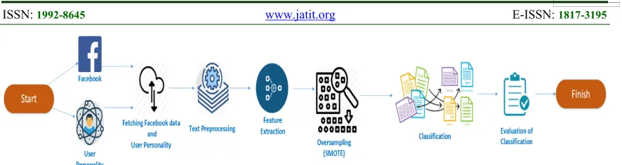
3. METHODOLOGY 3.1 The Concepts

The concept of methodology in this study is shown in Figure 1. Based on the illustration in Figure 1, the core steps of this study are as follows: a. Collecting datasets consisting of personality and

post values captured using the Facebook API; b. Pre-processing text data from Facebook wall

posts;

c. Extracting text feature on text data; d. Oversampling with SMOTE;

e. Classifying with SVM, Naïve Bayes and Logistic Regression;

f. Evaluating results from personality predictions.

3.2 Data Collection

At this stage, information from Facebook users, specifically their posts on their Facebook wall, was collected.

The process of data retrieval was conducted by using the Facebook API via online survey application created by the authors. The online survey app contains a personality measurement tool to determine the personality traits of Facebook users.

Before completing the online personality survey, users were required to log in and connect to their Facebook. After users had filled out the survey, the application would retrieve all information and Facebook posts on the users’ Facebook. Afterwards, the application would generate and display the results of personality traits.

The tool which was used to determine the personality is the Big Five Inventory, which consists of 44 items of questions measured using the Likert scale [23]. In order to accommodate the Indonesian Facebook users, the authors utilized the Indonesian translation of the Big Five Inventory from Ramdhani [24].

The online survey was then administered on Indonesian Facebook users across different ages and genders in the academic community.

By the end of data collection stage, 345 participants had filled the survey, and their personality labels were acquired. The responses and information collected from these 345 participants were used as the data for this research. Distribution of manually-gathered dataset from participants can be seen in Table 1.

Table 1. Distribution of Manually-Gathered Dataset

Trait Labels

Amount of

Participants _Total High

Trait Trait Low

Openness 281 64 345

Conscientiousness 260 85 345

Extraversion 245 100 345

Agreeableness 319 26 345

Neuroticism 197 148 345

3.3 Text Pre-Processing

At this stage, the texts would undergo the pre-processing step. This step is necessary for data cleansing process in order to ensure that the data are consistent and uniform before the features of the texts were extracted. The stages are shown in Figure 2.

6882

Figure 2 : Stages of Text Pre-Processing

a. Case Folding involves changing all the capital letters found either in the beginning, middle or end of the word into lowercase. For example, the sentence as shown below:

"Aku pernah Kehilangan Semuanya"

would be changed into:

"aku pernah kehilangan semuanya".

b. Tokenizing involves removing all the URLs, hashtags and punctuation found in sentences and separating all sentences into words. For example, the sentence as shown below:

"mungkin bisa di bagi ke teman, saudara dkk alamat survei :

https://docs.google.com/forms/d/12gzlkbuzwsd ssmxli6xv86kn8uzvqwrnvjsimd7ddcw/viewfor

m" would be changed into:

" mungkin bisa di bagi ke teman saudara dkk

alamat survei".

Then the sentence would be separated into words as follows: “mungkin”, “bisa”, “di”, “bagi”, “ke”, “teman”, “saudara”, “dkk”,

“alamat”, and “survei”.

c. Filtering involves removing words that are considered meaningless using the list of stopwords by Tala [25]. Furthermore, it also involves translating words from English into Indonesian. Non-standard Indonesian words

and slang language would be converted into formal Indonesian forms that comply with

Kamus Besar Bahasa Indonesia (Great

Dictionary of the Indonesian Language). For example, the sentence as shown below:

"akhirnya nemuin makanan ini gak berhenti

makan deh eating is a talent"

would be changed into:

"menemukan makanan tidak berhenti

makan deh makan adalah sebuah talenta".

d. Stemming is the process of eliminating affixes either at the beginning (e.g. me-, ber-, ter-, and so on) or at the end of a word (e.g. –kan, an, -i, and so on). For example, the sentence as shown below:

"menemukan makanan berhenti makan deh

makan adalah sebuah talenta"

would be converted into:

"temu makan henti makan deh makan adalah

sebuah talenta".

e. Text Normalization is the last step in text pre-processing which involves eliminating repetitive letters that cause the wording to be unstructured. Then, the filtering and stemming steps would be repeated before the step of removing one-letter character, which has no meaning, was applied. For example, the sentence as shown below:

"malam michael gilaaaaaaa Baaaaaangeeeeet

maju kocak a"

would be converted into:

"malam michael gila banget maju kocak".

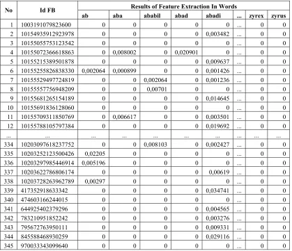
3.4 Text Feature Extraction

The feature extraction using TF-IDF resulted in attributes as much as 78.245 words. Despite the fact that the authors filtered the attributes beforehand using corpus generated by the authors themselves, the number of attributes which did not conform to the standard Indonesian language (e.g. abbreviations, slang language, and so on) was abundant.

6883

Table 2. Results of Feature Extraction

No Id FB Results of Feature Extraction In Words

ab aba ababil abad abadi ... zyrex zyrus

1 1003191079823600 0 0 0 0 0 ... 0 0

2 10154935912923978 0 0 0 0 0,003482 ... 0 0

3 10155055753123542 0 0 0 0 0 ... 0 0

4 10155072366618863 0 0,008002 0 0,020901 0 ... 0 0

5 10155215389501878 0 0 0 0 0,009637 ... 0 0

6 10155255826838330 0,002064 0,000899 0 0 0,001426 ... 0 0

7 10155529497724819 0 0 0,002064 0 0,001236 ... 0 0

8 10155557756948209 0 0 0,00701 0 0 ... 0 0

9 10155681265154189 0 0 0 0 0,014645 ... 0 0

10 10155691836128060 0 0 0 0 0 ... 0 0

11 10155709311850769 0 0,006617 0 0 0,003501 ... 0 0

12 10155788105797384 0 0 0 0 0,019692 ... 0 0

... ... ... ... ... ... ... ... ... ...

334 10203097618237752 0 0 0,008103 0 0,002427 ... 0 0

335 10203252123500426 0,02205 0 0 0 0 ... 0 0

336 10203297985446914 0,005196 0 0 0 0 ... 0 0

337 10203622786806174 0 0 0 0 0,00619 ... 0 0

338 10203728263962789 0,00297 0 0 0 0 ... 0 0

339 417352918633342 0 0 0 0 0,034741 ... 0 0

340 474603166244015 0 0 0 0 0 ... 0 0

341 644925402379296 0 0 0 0 0,004565 ... 0 0

342 783210951852242 0 0 0 0 0,003276 ... 0 0

343 795672763950111 0 0 0 0 0,009331 ... 0 0

344 845588468930259 0 0 0 0 0,029116 ... 0 0

345 970033343099640 0 0 0 0 0 ... 0 0

3.5 SMOTE (Synthetic Minority Oversampling Technique)

In this research, the SMOTE method was used to handle the problem of data imbalance in the dataset [17]. At this stage, new synthetic data in the class with low number of data were made. The process of creating synthetic data was conducted until the data in each class became balanced with the class that has the highest amount of data. SMOTE was performed after the feature extraction stage was completed, and the output of the SMOTE result was a new synthetic data. The parameters used in the SMOTE method were as follows:

a. The number of nearestNeighbors used is 5;

b. The number of randomSeed (the amount of generator used for oversampling) used is 1;

c. The percentage of SMOTE for each class to be balanced is 77% for Class O, 67% for Class C, 59% for Class E, 91% for Class A and 24% for Class N.

Results of datasets before and after using the SMOTE method are shown in Table 3.

Table 3. Distribution of Manually-Gathered Datasets Before and After Using SMOTE

Traits SMOTE Before SMOTE After Yes No Yes No

Openness 281 64 281 281

Conscientiousness 260 85 260 260 Extraversion 245 100 245 245 Agreeableness 319 26 319 319 Neuroticism 197 148 197 197

3.6 Model Classification

6884 classification of 1 and 0 for each class of personality. Next, we randomly split the datasets in 2 groups: training data and testing data. 90% of the dataset was used as training data while the remaining 10% was used as testing data. The whole process of classification used python libraries.

4. RESULTS

The accuracy results of the classification using SVM with Linear Kernel for every 10 attempts are shown in Table 4.

Table 4. The Accuracy Results of Classification Using SVM with Linear Kernel

Fold Traits(%)

Ope Con Ext Agr Neu 1 94,8 88,5 82,0 100,0 67,5 2 91,1 80,8 74,0 100,0 55,0 3 96,4 92,3 82,0 100,0 60,0 4 100,0 96,2 82,0 100,0 60,0 5 98,2 100,0 96,0 100,0 57,5 6 98,2 96,2 87,5 98,4 55,0 7 100,0 98,1 95,8 100,0 57,5 8 100,0 98,1 97,9 100,0 60,5 9 96,4 98,1 95,8 98,4 84,2 10 100,0 96,2 100,0 100,0 89,5 Avg 97,5 94,4 89,3 99,7 64,7

In Table 4, it can be seen that based on the result of classification using SVM with Linear Kernel, the trait of Agreeableness had the highest degree of average accuracy, which is 99,7%, and it can also be seen that the accuracy reached 100% in Fold 1, 2, 3, 4, 5, 7 , 8 and 10. Meanwhile, the trait of Neuroticism had the lowest degree of average accuracy, which is only 64,7%, and it can be noted as well that the lowest accuracy (55,0%) was in Fold 2 and 6.

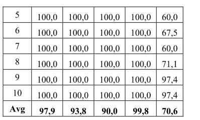
The accuracy results of the classification using SVM with RBF Kernel for every 10 attempts are shown in Table 5.

Table 5. The Accuracy Results of Classification Using SVM with RBF Kernel

Fold Traits(%)

Ope Con Ext Agr Neu 1 _{93,1 78,8 76,0 98,4 60,0} 2 _{89,3 76,9 82,0 100,0 57,5} 3 _{96,4 88,5 70,0 100,0 62,5} 4 _{100,0 94,2 72,0 100,0 72,5}

5 _{100,0 100,0 100,0 100,0 60,0} 6 _{100,0 100,0 100,0 100,0 67,5} 7 _{100,0 100,0 100,0 100,0 60,0} 8 _{100,0 100,0 100,0 100,0 71,1} 9 _{100,0 100,0 100,0 100,0 97,4} 10 _{100,0 100,0 100,0 100,0 97,4} Avg _{97,9 93,8 90,0 99,8 70,6}

In Table 5, it can be seen that based on the result of classification using SVM with RBF kernel, the trait of Agreeableness had the highest degree of average accuracy, which is 99,8%, and it can also be seen that the accuracy reached 100% in Fold 2 to 10. Meanwhile, the lowest average accuracy was the trait of Neuroticism with the average accuracy of 70,6%, and it can also be seen that the lowest accuracy (57,5%) was in Fold 2.

The accuracy results of the classification using SVM with Polynomial Kernel for every 10 attempts are shown in Table 6.

Table 6. The Accuracy Results of Classification Using SVM with Polynomial Kernel

Fold Traits(%)

Ope Con Ext Agr Neu 1 _{94,8 92,3 84,0 100,0 62,5} 2 _{91,1 80,8 86,0 100,0 50,0} 3 _{98,2 90,4 82,0 100,0 62,5} 4 _{100,0 98,1 78,0 100,0 70,0} 5 _{96,4 100,0 100,0 100,0 60,0} 6 _{100,0 100,0 100,0 100,0 65,0} 7 _{100,0 100,0 100,0 100,0 60,0} 8 _{96,4 100,0 100,0 100,0 73,7} 9 _{100,0 100,0 100,0 100,0 97,4} 10 _{96,4 100,0 100,0 100,0 97,4} Avg _{97,3 96,2 93,0 100,0 69,8}

The results in Table 6 shows that by using SVM with Polynomial kernel, the highest average accuracy belongs to the trait of Agreeableness (100%), and it is important to note that the accuracy reached 100% in Fold 1 to 10. On the other hand, the lowest average accuracy belongs to the trait of Neuroticism (69,8%), and it can also be seen that the lowest accuracy of 50% was in Fold 2.

6885

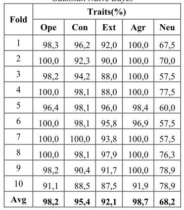
Table 7. The Accuracy Results of Classification Using Gaussian Naive Bayes

Fold Traits(%)

Ope Con Ext Agr Neu 1 _{98,3 96,2 92,0 100,0 67,5} 2 _{100,0 92,3 90,0 100,0 70,0} 3 _{98,2 94,2 88,0 100,0 57,5} 4 _{100,0 98,1 88,0 100,0 77,5} 5 _{96,4 98,1 96,0 98,4 60,0} 6 _{100,0 98,1 95,8 96,9 57,5} 7 _{100,0 100,0 93,8 100,0 57,5} 8 _{100,0 98,1 97,9 100,0 76,3} 9 _{98,2 90,4 91,7 100,0 78,9} 10 _{91,1 88,5 87,5 91,9 78,9} Avg _{98,2 95,4 92,1 98,7 68,2}

Based on the results in Table 7, by using Gaussian Naïve Bayes, the highest average accuracy belongs to the trait of Agreeableness with the average accuracy of 98,7%. In addition, it is important to note that the accuracy reached 100% in Fold 1, 2, 3, 4, 7, 8 and 9. Meanwhile, the lowest average accuracy belongs to the trait of Neuroticism with the average accuracy of 68,2%, and it can also be seen that the lowest accuracy (57,5%) was in Fold 3, 6 and 7.

The accuracy results of the classification using Logistic Regression for every 10 attempts are shown in Table 8.

Table 8. The Accuracy Results of Classification Using Logistic Regression

Fold Traits(%)

Ope Con Ext Agr Neu 1 _{91,4 80,8 70,0 96,9 62,5} 2 _{64,3 67,3 66,0 100,0 57,5} 3 _{83,9 84,6 64,0 100,0 55,0} 4 _{98,2 92,3 70,0 100,0 55,0} 5 _{85,7 100,0 92,0 100,0 50,0} 6 _{92,9 94,2 83,3 100,0 57,5} 7 _{96,4 94,2 89,6 100,0 52,5} 8 _{94,6 92,3 93,8 100,0 57,9} 9 _{94,6 96,2 85,4 98,4 81,6} 10 _{92,9 94,2 97,9 100,0 76,3} Avg 89,5 89,6 81,2 99,5 60,6

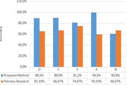
Based on the results on Table 8 above, it is evident that by using Logistic Regression, the highest average accuracy belongs to the trait of Agreeableness with the average accuracy of 99,5%, and the accuracy in fact reached 100% in Fold 2, 4, 5, 6, 7, 8, and 10. On the other hand, the lowest average accuracy belongs to the trait of Neuroticism (60,6%) in which the lowest accuracy, which is 50%, was in Fold 5.

The results explained above would be compared to the results of research by Tandera et al. Tandera et al also used SVM, Gaussian Naïve Bayes, and Logistic Regression as their classification algorithm. For the comparison on accuracy, two scenarios were employed. For the first scenario, datasets from myPersonality website were used while for the second scenario, the authors used datasets which are collected manually as conducted by Tandera et al [5].

The comparison on the accuracy results for the first scenario using SVM algorithm is shown in Figure 3. In this case, the authors used SVM with Polynomial Kernel for the proposed method.

Figure 3 : Comparison on Accuracy Result Using SVM with Polynomial Kernel for First Scenario

6886

Figure 4 : Comparison on Accuracy Result Using Gaussian Naïve Bayes for First Scenario

The comparison on the accuracy results for the first scenario using Logistic Regression for the proposed method is shown in Figure 5.

Figure 5 : Comparison on Accuracy Result Using Logistic Regression for First Scenario

Based on Figure 3, 4 and 5, for the first scenario, the traits of Openness, Conscientiousness, Extraversion and Agreeableness show significant increase in accuracy when compared to the previous study. However, the trait of Neuroticism only shows slight increase in accuracy.

The comparison on the accuracy results for the second scenario using SVM algorithm is shown in Figure 6. In this case, the authors used SVM with Polynomial Kernel for the proposed method.

Figure 6 : Comparison on Accuracy Result Using SVM with Polynomial Kernel for Second Scenario

The comparison on accuracy results for the second scenario using Gaussian Naïve Bayes for the proposed method is shown in Figure 7.

Figure 7 : Comparison on Accuracy Result Using Gaussian Naïve Bayes for Second Scenario

The comparison on accuracy results for the second scenario using Logistic Regression for the proposed method is shown in Figure 8.

Figure 8 : Comparison on Accuracy Result Using Logistic Regression for Second Scenario

Similar to the first scenario, there is significant increase in accuracy for the traits of Openness, Conscientiousness, Extraversion and Agreeableness. However, the trait of Neuroticism using SVM with Polynomial Kernel shows only slight increase by 0,47% in accuracy. Meanwhile, the method used in previous study exhibits better accuracy than the proposed method when Gaussian Naïve Bayes and Logistic Regression algorithm were used.

5. CONCLUSION

6887 model with Linear, Polynomial and RBF kernels, and Gaussian Naïve Bayes and Logistic Regression has an excellent accuracy in predicting the personality. In predicting personality traits of Openness, Conscientiousness, Extraversion and Agreeableness have an average accuracy rate above 80%. It also proves that the SMOTE algorithm works well in dealing with the issue of data imbalance.

In addition, the accuracy of this study was also compared to the results of research conducted by Tandera et al using 2 scenarios: by using datasets from myPersonality website and by using manually-collected datasets.

From the comparison for the first scenario, it can be concluded that the proposed method was successful in increasing the accuracy of personality prediction for all classification models. Moreover, it can be seen that there is significant increase in accuracy, especially in the trait of Openness. By using the Gaussian Naïve Bayes classification model, the trait of Openness reached the highest accuracy of 98,2%.

In the second scenario, the comparison of accuracy results also shows similar phenomenon in which there is significant increase in accuracy level in the traits of Openness, Conscientiousness, Extraversion and Agreeableness. The highest accuracy in the second scenario is the trait of Openness using Gaussian Naïve Bayes in which the accuracy rate reached 98,2%. However, compared to the trait of Openness, there is no increase in accuracy for the trait of Neuroticism from using Gaussian Naïve Bayes and Logistic Regression. It could be seen from the fact that by using the proposed method, the accuracy for the trait of Neuroticism only reached 68,2% whereas the result of the previous research reached 70%.

REFRENCES:

[1] J. V. Haxby, E. A. Hoffman, and M. I. Gobbini, “The distributed human neural system for face perception,” Trends Cogn. Sci., vol. 4, no. 6, pp. 223–233, 2000. [2] S. Poria, A. Gelbukh, and B. Agarwal,

“Common Sense Knowledge Based Personality Recognition from Text,” pp. 484–485, 2013.

[3] E. El Sayed, “Exploiting Social Annotations for Personalizing Retrieval,” vol. 10, no. 6, pp. 192–202, 2017.

[4] B. Y. Pratama and R. Sarno, “Personality Classification Based on Twitter Text Using Naive Bayes , KNN and SVM,” pp. 170– 174, 2015.

[5] T. Tandera et al., “Personality Prediction System from Facebook Users,” Procedia

Comput. Sci., vol. 116, pp. 604–611, 2017.

[6] W. Andangsari and M. N. Suprayogi, “Personality Prediction Based on Twitter Information in Bahasa Indonesia,” Proc.

Fed. Conf. Comput. Sci. Inf. Syst., vol. 11,

pp. 367–372, 2017.

[7] H. Sain and S. Wulan, “Combine Sampling Support Vector Machine for Imbalanced Data Classification,” Procedia - Procedia

Comput. Sci., vol. 72, pp. 59–66, 2015.

[8] J. Ahmad, F. Javed, and M. Hayat, “Artificial Intelligence in Medicine Intelligent computational model for classification of sub-Golgi protein using oversampling and fisher feature selection methods,” Artif. Intell. Med., vol. 78, pp. 14– 22, 2017.

[9] J. Pednekar and S. Dubey, “Identifying Personality Trait using Social Media : A Data Mining Approach,” Int. J. Curr. Trends

Eng. Res., vol. 2, no. 4, pp. 489–496, 2016.

[10] B. Agarwal, “Personality Detection from Text : A Review,” Int. J. Comput. Syst., vol. 1, no. 1, pp. 1–4, 2014.

[11] M. Kosinski and D. Stillwell, “Personality and Patterns of Facebook Usage,” 2012. [12] K. Peng, L. Liou, C. Chang, and D. Lee,

“Predicting Personality Traits of Chinese Users Based on Facebook Wall Posts,” 2015.

[13] J. Golbeck, “Predicting Personality with Social Media,” Proc. 2011 Annu. Conf. Ext. Abstr. Hum. factors Comput. Syst. CHI EA 11, pp. 253–262, 2011.

[14] R. Talib, M. K. Hanif, S. Ayesha, and F. Fatima, “Text Mining : Techniques , Applications and Issues,” Int. J. Adv.

Comput. Sci. Appl., vol. 7, no. 11, pp. 414–

418, 2016.

[15] S. A. Salloum, M. Al-Emran, and K. Shaalan, “A Survey of Text Mining in Social Media : Facebook and Twitter Perspectives,” Adv. Sci. Technol. Eng. Syst. J., vol. Vol. 2, No, no. January, 2017. [16] T. Mardiana, R. D. Nyoto, P. Studi, and T.

Informatika, “Kluster Bag-of-Word Menggunakan Weka,” vol. 1, no. 1, pp. 1–5, 2015.

6888 16, pp. 321–357, 2002.

[18] Y. E. Achyani, “Prediksi Pemasaran Langsung Menggunakan Metode Support Vector Machine,” vol. III, no. 2, pp. 2–7, 2017.

[19] M. Abdi, D. Herumurti, and I. Kuswardayan, “Analisis perbandingan kecerdasan buatan pada computer player dalam mengambil keputusan pada game battle RPG,” vol. 15, pp. 226–237, 2017.

[20] A. A. Haritama, “Penerapan Model Mesin Belajar Support Vector Machines pada Automatic Scoring Untuk Jawaban Singkat,” Universitas Atma Jaya Yogyakarta, 2017.

[21] M. I. Jambak and P. S. Setiawan, “The Development Of Bahasa Indonesia Corpora For Machine Learning Model In Combating Cyber Bullying : A Case Study Of The Indonesian 2017 Capital City Governor Election,” J. Theor. Appl. Inf. Technol., vol. 96, no. 7, pp. 1971–1988, 2018.

[22] B. Kurniawan, M. A. Fauzi, and A. W. Widodo, “Klasifikasi Berita Twitter Menggunakan Metode Improved Naïve Bayes,” vol. 1, no. 10, pp. 1193–1200, 2017. [23] R. John, T. Big-five, and L. A. Pervin, “Big

Five Inventory ( BFI ),” vol. 2, 1999. [24] N. Ramdhani, “Adaptasi Bahasa dan Budaya

Inventori Big Five,” vol. 39, no. 2, pp. 189– 207, 2012.