Outlier Detection in Local Level Model: Impulse Indicator Saturation Approach

(1)

Outlier Detection in Local Level Model: Impulse

Indicator Saturation Approach

F. Z. Che Rose1,2,*_{, M.}_{T. Ismail}2_{, N. A. K. Rosili}1

1_{School of Computing, Faculty of Science and Technology, Quest International University Perak, Malaysia} 2_{School of Mathematical Sciences, Universiti Sains Malaysia, Malaysia}

Received July 1, 2019; Revised September 3, 2019; Accepted September 14, 2019

Abstract The existence of outliers in financial time

series may affect the estimation of economic indicators. Detection of outliers in structural time series framework by using indicator saturation approach has become our main interest in this study. The reference model used is local level model. We apply Monte Carlo simulations to assess the performance of impulse indicator saturation for detecting additive outliers in the reference model. It is found that the significance level, α = 0.001 (tiny) outperformed the other target size in detecting various size of additive outliers. Further, we apply the impulse indicator saturation to detection of outliers in FTSE Bursa Malaysia Emas (FBMEMAS) index. We discover that there were 14 outliers identified corresponding to several economic and financial events.

Keywords Outliers, Local Level, Indicator Saturation,

Monte Carlo, Impulse Indicator Saturation, Structural Time Series

1. Introduction

Financial time series usually have abnormal events over time that may affect the estimation of the economic indicator. The impact of the events is often overlooked. One important issue is the detection procedure in the time series. Outliers refer to the abnormal observation that may arise because of measurement error or short-term changes in the underlying process. As noted by [1], the outlier causes an immediate and one-shot effect on the observed series. Previous work was done by [2] to identify the locations and types of outliers in a time series. Then, several studies have been made by [3] and [4] shows that their approach quite effective in detecting the locations and estimating the effects of huge isolated outliers. Then, [5] demonstrated the new and convenient procedure to test for

an unknown number of breaks, occurring at unknown times with unknown durations and magnitudes. The procedure is known as impulse-indicator saturation (IIS) where it relies on the addition of a dummy pulse for each observation in the series. A recent study was done by [6] draws our attention to the fact that it was the first study to detect outlier in structural time series model, specifically basic structural model (BSM) using indicator saturation approach. However, in this paper, we take a new look to apply the indicator saturation approach in structural time series proposed by [7]. The reference model is the local level deterministic and local level stochastic model. This study aims to contribute to the literature lies in the fact that it is the first to use local level model with indicator saturation approach to outlier detection. In addition, this study provides an exciting opportunity to advance our knowledge outlier detection using indicator saturation approach in structural time series framework. Our main interest in empirical applications lies in the capability of indicator saturation approach to identify potential outlier corresponding to the economic and financial crisis happened at the end of 2008.

The remainder of this paper organized as follows. Section 2 describes the general knowledge of the reference model, the concept of indicator saturation and Monte Carlo simulations to assess the performance of indicator saturation approach, summarizing our findings on the performance of IIS with both local models. Then, we applied IIS to real data for detecting outliers. Section 3 concludes.

2. Materials and Methods

2.1. Local Level Model

(2)

both level and slope to be stochastic. The local level model can be described as follows:

2

~ (0, )

t t t t

y =

µ ε ε

+ NID

σ

ε (1)

2

1 ~ (0, )

t t t t NID ξ

µ₊ =µ ξ+ ξ σ (2)

for t=1,...,n, where

µ

_t is the unobserved level at time t,

t

ε

is the observation disturbance at time t or irregular component and

ξ

_t is the level disturbance at time t. The observation and level disturbances are all assumed to be serially and mutually independent and normally distributed with zero mean and variances

σ

ε2 and

σ

ξ2 respectively. Equation (1) is called observation equation and (2) is known as state equation. When the state disturbances are all fixed on

σ

_ξ2

=

0

for

t

=

1,...,

n

the model reduces to a deterministic model where the level does not vary over time. On the other hand, when the level is allow to vary over time it is treated as stochastic process.

2.2. Indicator Saturation

Indicator saturation consider a general-to-specific approach according to which indicator variables were added based on the number of observations, T. [5] introduced IIS as a procedure for testing parameter constancy. In details, IIS is a generic test for an unknown number of breaks, occurring at unknown times anywhere in the sample with unknown magnitude and functional form. Further works about indicator saturation has been done by [6-10]. The applications of IIS in economic data have been done by [11- 13]. We employ impulse indicator saturation (IIS) in this study for outlier detection in the series. IIS is beneficial for detecting crises, jumps, and changes in financial time series. It also provides a framework for creating near real time early warning and rapid detection devices. In IIS framework, we denote

I

_t

( )

t

as a pulse dummy which equal to 1 for

t

=

t

and 0 otherwise. We adopt the split-half approach to integrate IIS into the model

y

_t

=

µ ε

_t

+

_t

, 1,...,

t

=

T

where

ε

_t is normally and independently distributed with mean zero and variance 2

ε

σ

. The integration of IIS will give an augmented block of impulse indicators as follows:

2

1

( )

, 1,...,

T

t lk t t

k

y

µ

δ

I k

ε

t

T

=

= +

∑

+

=

Split-half approach begins with an amount of

T

₂

indicators are added to the model for the first half of the sample. Any indicator in the analysis with t-value less than significance level, α will be omitted. Next, the

procedure is repeated with the second T−T₂indicators. Finally, terminal model consist of two sets of significant dummies is re-estimated to get the final model. IIS identify outliers with difference sign and magnitude in the series. All computations are performed using PcGive module in OxMetrics 8 (64 bit version).

2.3. Monte Carlo Simulation

Firstly, we generate time series according to both local level deterministic model and local level stochastics model respectively. As regards the simulation settings, the following specifications are considered for both models:

 The variance of parameter 2

₁

ε

σ

=

and

σ

_η2

=

0

for the local level deterministic model.

 The variance of parameter

σ

ε2

=

1

and

2

_0.001

η

σ

=

for the local level stochastic model.

 Various sample size used began with T = 500, 1000 and 2000 observations.

 Target size or significance level, α = 0.0001, 0.001, 0.01 and 0.025 which were labelled as minute, tiny, small and medium respectively. According to [13], these values will determine the statistical tolerance of the procedure. For example, a target of 0.01 for IIS indicates that on average we accept 1 impulse dummy that may not be in the data generating process for every 100 observations.

 We denoted the size of an outlier as kσ where k is an integer and σ is standard deviation of the series. Both positive and negative different magnitude of additive outliers (AO) were added in generated series commencing with the size of 4σ,6σ,7σ,8σ,10σ,12σ and 14σ. As reference to [6], we therefore set 7σ as benchmark value that determine the size of outlier. All these outliers were located randomly based on a random number generator.

2.3.1. Assessing the Performance of Impulse Indicator Saturation (IIS)

Confusion matrix was used in this study to summarize the outcome of single Monte Carlo simulation as employed by [6]. This table is used to describe the performance of a model on each set of generated series for which the true values of additive outliers (AO) are known. Confusion matrix can be illustrated as follows:

Actual Decision

No outlier Outlier Total No outlier A B T-n

Outlier C D n

(3)

A and D are identified as the number of correct decisions for both cases of no outlier and outliers at specified locations respectively. On the other hand, B and C denote the number of false decisions when no outlier appeared and when there are outliers at specified locations respectively. Meanwhile, n refers to the number outliers and T is the total observations in the series. Based on the confusion matrix, we employ the concepts of potency and gauge to determine the efficiency of the indicator saturation procedure. Potency is also known as sensitivity obtained by the ratio of D/n. Meanwhile, gauge or known as false positive rate is defined as B/(T-n). In addition, the

performance of IS also measured by accuracy rate which defined as (A+D)/T.

2.4. Results and Discussion

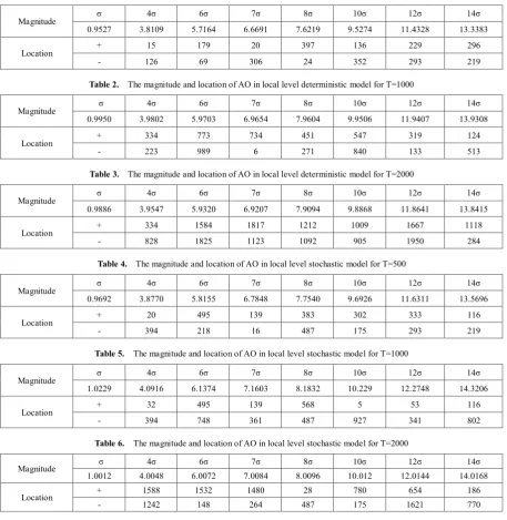
[image:3.595.70.528.242.711.2]

As mentioned earlier, we began the simulation procedures with three different numbers of observations for both local level models to demonstrate the ability of IIS in detecting outliers in each series. The locations of AO were predetermined by a random number generator as presented in Table 1-6 below.

Table 1. The magnitude and location of AO in local level deterministic model for T=500

Magnitude σ 4σ 6σ 7σ 8σ 10σ 12σ 14σ

0.9527 3.8109 5.7164 6.6691 7.6219 9.5274 11.4328 13.3383

Location + 15 179 20 397 136 229 296

- 126 69 306 24 352 293 219

0.9950 3.9802 5.9703 6.9654 7.9604 9.9506 11.9407 13.9308

Location + 334 773 734 451 547 319 124

- 223 989 6 271 840 133 513

0.9886 3.9547 5.9320 6.9207 7.9094 9.8868 11.8641 13.8415

Location + 334 1584 1817 1212 1009 1667 1118 - 828 1825 1123 1092 905 1950 284

Table 4. The magnitude and location of AO in local level stochastic model for T=500

0.9692 3.8770 5.8155 6.7848 7.7540 9.6926 11.6311 13.5696

Location + 20 495 139 383 302 333 116

- 394 218 16 487 175 293 219

1.0229 4.0916 6.1374 7.1603 8.1832 10.229 12.2748 14.3206

Location + 32 495 139 568 5 53 116

- 394 748 361 487 927 341 802

1.0012 4.0048 6.0072 7.0084 8.0096 10.012 12.0144 14.0168

(4)

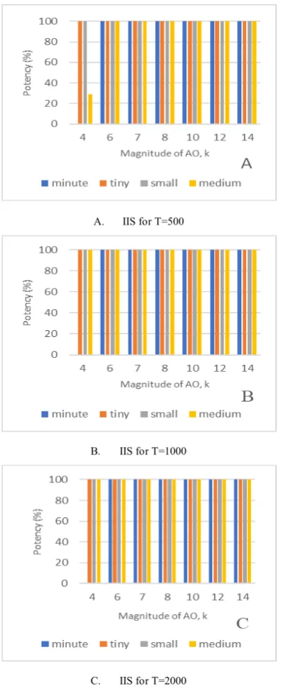
The effectiveness of indicator saturation procedure is assessed using the concepts of potency and gauge. The simulation results show that IIS is effective to capture almost 100% the outliers for various value of α, as well as small error rate. Interestingly, we found that different values of α and magnitude of AO affect the potency rate for all series in both local level models. This facilitates comparisons with [6] as the performance of IIS depends strongly on the magnitude of the outlier. When α = 0.0001 (minute), we found that at 4σ the potency at the lowest level for all series in both models. On the other hand, we found that the potency achieved 100% for all cases in both local level models as depicted in Fig. 1 and 2.

A. IIS for T=500

B. IIS for T=1000

C. IIS for T=2000

Figure 1. The potency rate with various size of AO for local level deterministic model

A. IIS for T=500

B. IIS for T=1000

C. IIS for T=2000

Figure 2. The potency rate with various size of AO for local level stochastic model

[image:4.595.317.524.64.594.2] [image:4.595.74.278.236.733.2]

(5)

A. IIS for T=500

B. IIS for T=1000

C. IIS for T=2000

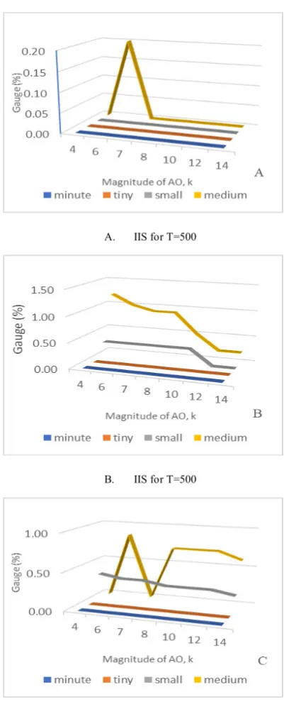
Figure 3. The gauge rate with various size of AO for local level deterministic model

A. IIS for T=500

B. IIS for T=500

C. IIS for T=500

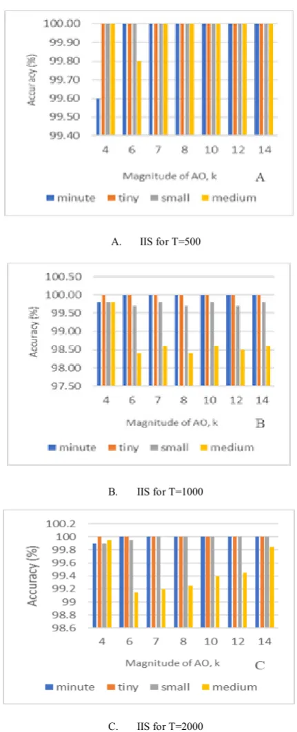
[image:5.595.320.521.71.577.2] [image:5.595.73.279.76.585.2]

(6)

In view of accuracy of the model, we found remarkable results when α = 0.001 (tiny) is applied. Overall, the accuracy rate is still above 98% for different values of significance level, α, magnitude and location of AO. As the number of observations, T increase we found that the accuracy rate reduces by 1% when the target size at medium level as depicted in Fig. 5B and 5C.

A. IIS for T=500

B. IIS for T=1000

C. IIS for T=2000

Figure 5. The accuracy rate with various size of AO for local level deterministic model

A. IIS for T=500

B. IIS for T=1000

C. IIS for T=2000

Figure 6. The accuracy rate with various size of AO for local level stochastic model

2.5. Empirical Application

[image:6.595.313.529.75.607.2] [image:6.595.65.284.166.701.2]

(7)

2008, until May 21, 2019 (2333 observations) provided by Datastream. We aim to assess the application of IIS in detecting financial crises, recession’s period and government policy changes along the estimation period.

[image:7.595.57.292.231.363.2]

Figure 7 & 8 below portrayed the daily closing price and return series for FBMEMAS. We used return series in outlier detection procedure which shows the natural logarithm of the difference between the closing price index and the value for the corresponding price of the preceding day. The series then multiplied by 100 to ease interpretation and avoid numerical error from original return series.

[image:7.595.59.292.394.527.2]

Figure 7. The closing price of FTSE Bursa Malaysia Emas index

Figure 8. Return series of FTSE Bursa Malaysia Emas index Table 7 below illustrates the result of IIS procedure for FBMEMAS. We found there were 20 outliers captured in the series by IIS procedure. We can relate there are various events that can be associated with FBMEMAS for example global financial crisis in 2008-2009. Interestingly, we may relate the event on 8 Aug 2011 refers to Black Monday where United States (US) and the global stock market crashed due to downgraded credit rating given by Standard & Poors to US sovereign debt from AAA to AA+. As regard to Black Monday, it can be seen that in Figure 7 the closing price plunged by 250 points from the closing price on Friday for FBMEMAS. Besides, the US debt ceiling crisis in 2013 and declination of international crude oil prices also can be associated with FBMEMAS index movement. Therefore, we concluded that FBMEMAS index was affected by various global events around the world.

Table 7. Specific date of outliers detected by IIS

No. of outliers

detected Specific Date

16

10 Oct 2008, 24 Oct 2008, 3 Nov 2008, 8 Aug 2011, 22 Sept 2011, 26 Sept 2011, 21 Jan 2013, 6 May 2013, 13 June 2013, 20 Aug 2013, 1 Dec 2014, 15 Dec 2014, 12 Aug 2015, 24 Aug 2015,

4 Jan 2016, 6 Feb 2018

3. Conclusions

This study intended to investigate the performance of the indicator saturation approach specifically IIS a new methodology to detect outliers in local level models. Since there is no study yet been investigated, we implemented IIS in the framework of both local level deterministic and local level stochastic models. The IIS was customized to detect AOs as been done previously by [6]. Then, the effectiveness of IIS was evaluated by several indicators that are potency, gauge, and accurate rate. We also found that the location of AO influenced the performance of IIS strongly with the gauge values rise when the AO appears at the beginning or the end of the series in the simulation. Besides, we found that the difference value of the target size also affects the potency and gauge. We concluded that a target size α = 0.001 outperformed the other target size.

In the final section of this article, we applied IIS to the FBMEMAS index time series using target size α = 0.001. The result demonstrates that there are 16 outliers detected in the series which most of them were strongly associated with global economic events. This study do not consider the presence of structural breaks in the data. However, future research can be conducted to the detection of outlier and structural breaks using indicator saturation approach.

Acknowledgements

The authors would like to extend their sincere gratitude to the Ministry of Higher Education Malaysia (MOHE) for the financial supports received for this work under FRGS grant (203/PMATHS/6711604).

REFERENCES

C. Chen, L. M. Liu. Joint Estimation of Model Parameters [1]

and Outlier Effects in Time Series, Journal of American Statistical Association., Vol. 88, No. 421, 284-297, 1993. G. E. P. Box, G. C. Tiao. Intervention Analysis with [2]

Applications to Economic and Environmental Problems, Journal of American Statistical Association. Vol. 70, No. 349, 70–79, 1975.

I. Chang, G. C. Tioa, C. Chen. Estimation of Time Series [3]

(8)

Vol.30, No.2, 193-204, 1988.

R. S. Tsay. Outliers, Level Shifts, and Variance Changes in [4]

Time Series, Journal of Forecasting, Vol. 7, No. 1, 1–20, 1988.

D. F. Hendry. An econometric analysis of US food [5]

expenditure, 1931-1989 in Methodlogy and tacit knowledge: two experiments in econometrics in econometrics, 341-361, John Wiley and Sons, England, 1999.

M. Marczak, T. Proietti. Outlier detection in structural time [6]

series models: The indicator saturation approach, International Journal of Forecasting, Vol. 32, No. 1, 180– 202, 2016.

S. Johansen, B. Nielsen. An Analysis of the Indicator [7]

Saturation Estimator as a Robust Regression Estimator in The Methodology and Practice of Econometrics: A Festschrift Honour David F. Hendry, 1-36, Oxford University Press, England 2009.

J. L. Castle, J. A. Doornik, D. F. Hendry, and F. Pretis. [8]

Detecting Location Shifts by Step-indicator Saturation, Econometrics, Vol. 3, No. 2, 240–264, 2015.

J. A. Doornik, D. F. Hendry, and F. Pretis. Step-indicator [9]

saturation, Oxford Economic Department Discussion Paper No. 658, 2013.

C. Santos, D. F. Hendry, and S. Johansen. Automatic [10]

selection of indicators in a fully saturated regression. Computational Statistics, Vol. 23, No. 2, 317–335, 2008. D. F. Hendry, G. E Mizon. Econometric Modelling of Time [11]

Series with Outlying Observations, Journal of Time Series Econometrics, Vol. 3. No.1, 2011.

N. R. Ericsson. How biased are U.S. government forecasts of [12]

the federal debt?, International Journal of Forecasting, Vol. 33, No. 2, 543–559, 2017.

R. Mariscal, A. Powell. Commodity Price Booms and [13]