Simulation of the Lock Exchange Hydraulics using the Discontinuous Galerkin Method

Simulation of the Lock-Exchange Hydraulics Using the

Discontinuous Galerkin Method

Nouh Izem

EMMS Faculty of science, Ibn Zohr University Agadir,

Morocco

Mohammed Seaid

of Durham, South Road, Durham DH1 3LE, UK

Mohamed Wakrim

Zohr University Agadir, Morocco

ABSTRACT

Numerical simulations of the lock-exchange hydraulics have been carried out using a discontinuous Galerkin finite element method. The basic water circulation in the lock-exchange hydraulics consists in an upper layer of cold, fresh surface water and an opposite deep current of warmer, salty outflowing water. The governing equations are the well-established two-layer shallow water system including bathymetric forces. The considered discontinuous Galerkin method is a stable, highly accurate and locally conservative finite element method whose approximate solutions are discontinuous across interelement boundaries; this property renders the method ideally suited for the hp-adaptivity. The proposed method can handle complex topography using unstructured grids and it satisfies the conservation property. Several numerical results are presented to demonstrate the high resolution of the proposed method and to confirm its capability to provide accurate and efficient simulations for the lock-exchange hydraulics.

Keywords

Discontinuous Galerkin method; Two-layer shallow water equations; Finite element; Lock-exchange hydraulics.

1.

INTRODUCTION

During the last decades partial differential equations have been used as practical tools to model many environmental problems from real life. They have also been used to approximate and predict the dynamics of such problems. The goal of the present work is to provide a highly accurate and practical numerical model able to resolve and correctly capture the lock-exchange hydraulics. The water flow is governed by the depth-averaged Navier-Stokes equations involving several assumptions including (i) the domain is shallow enough to ignore the vertical effects, (ii) the pressure is hydrostatic, and (iii) viscous dissipation of the energy is ignored. These shallow water equations in depth-averaged form have been successfully applied to many engineering problems and their application fields include a wide spectrum of phenomena other than water waves. For instance, the shallow water equations have applications for tidal flows in an estuary or coastal regions, rivers, reservoirs and open channel flows. Such practical flow problems are not trivial to simulate since the geometry can be complex and the topography irregular. On the other hand, single-layer shallow water equations have the drawback of missing some physical dynamics in the vertical motion. Therefore, during the past years, multi-layer shallow water models have been attracted more attention and have became a very useful tools to solve hydrodynamical flows such as rivers, estuaries, bays and other

nearshore regions where water flows interact with the bed geometry and wind shear stresses, see for instance [12, 5, 22, 1, 10, 23]. The layers can be formed in the shallow water model based on the vertical variation of water density which in general depends on the water temperature and water salinity. The main advantage of these models is the fact that the two-layer shallow water model avoids the expensive three-dimensional Navier-Stokes equations and obtains stratified horizontal flow velocities as vertical velocities are relatively small and the flow is still within the shallow water regime. Accurate modeling of the lock-exchange hydraulics requires numerical methods capable of capturing highly advective flows and multi-scale features of the solution. The emphasis of the present work is on the application of the so-called nodal Discontinuous Galerkin (DG) methods to the lock-exchange hydraulics. The nodal DG method first introduced by Hesthaven and Warburton [16] for electro-dynamic simulations utilizes a nodal Lagrange interpolation basis as the approximating basis functions, which provides a simple and generic means to treat a (nonlinear) flux term appearing in the hyperbolic conservation laws. In recent years, a multitude of DG formulations has found rapid applications in many fields, for a review we refer to [6, 8] and further references are therein. The DG method has been successfully applied to the standard single-layer shallow water equations, see for example [2, 11, 21, 14]. However, the presence of nonconservative product terms in their two-layer counterpart poses serious numerical problems and at present there is no literature available how to genuinely solve the two-layer shallow water equations in a DG context, which motivated the research discussed in this article. Results presented in this paper show high resolution of the proposed DG method and confirm its capability to provide robust and accurate simulations for two-layer shallow water flows including complex topography.

The structure of this paper is as follows. In section 2, we present the mathematical equations for the two-layer shallow water equations used to model the lock-exchange hydraulics. The formulation of the DG method is detailed in section 3. This section includes the finite element discretization, the formulation of the weak form, numerical fluxes, and the time integration scheme. Section 4 is devoted to numerical results and applications. Finally, section 5 contains the conclusions.

2.

Governing Equations for Two-layer

Shallow Water Problems

𝜕ℎ1

𝜕𝑡 + 𝜕(ℎ1𝑢1)

𝜕𝑥 + 𝜕(ℎ1𝑣1)

𝜕𝑦 = 0, 𝜕(ℎ 1𝑢1)

𝜕𝑡 + 𝜕 𝜕𝑥 ℎ 1𝑢1

2₊1 2𝑔ℎ 1

2 ₊ 𝜕

𝜕𝑦(ℎ1𝑢1𝑣1) =

−𝑔ℎ1_𝜕𝑥𝜕 (ℎ2+ 𝐵), 𝜕(ℎ1𝑣1)

𝜕𝑡 + 𝜕

𝜕𝑥(ℎ1𝑢1𝑣1) + 𝜕 𝜕𝑦 ℎ1𝑣1

2₊1 2𝑔ℎ1

2 ₌

−𝑔ℎ1_𝜕𝑦𝜕 (ℎ2+ 𝐵),

(1)

𝜕ℎ2

𝜕𝑡 + 𝜕(ℎ2𝑢2)

𝜕𝑥 + 𝜕(ℎ2𝑣2)

𝜕𝑦 = 0, 𝜕(ℎ2𝑢2)

𝜕𝑡 + 𝜕 𝜕𝑥 ℎ2𝑢2

2₊1 2𝑔ℎ2

2 ₊ 𝜕

𝜕𝑦(ℎ2𝑢2𝑣2) =

−𝑔ℎ2_𝜕𝑥𝜕 𝜌_𝜌1

2ℎ1+ 𝐵 , 𝜕(ℎ2𝑣2)

𝜕𝑡 + 𝜕

𝜕𝑥(ℎ2𝑢2𝑣2) + 𝜕

𝜕𝑦 ℎ2𝑣22+ 1 2𝑔ℎ2

2 ₌

−𝑔ℎ2_𝜕𝑦𝜕 𝜌_𝜌1

2ℎ1+ 𝐵 ,

(2)

where the subscripts 1 and 2 represent respectively, the upper and lower layer in the hydraulic system. In the equations (1)-(2), 𝜌𝑗 is the water density of the jth layer, ℎ𝑗(𝑥, 𝑦, 𝑡) is the water height of the jth layer, 𝑢𝑗(𝑥, 𝑦, 𝑡) and 𝑣𝑗(𝑥, 𝑦, 𝑡) are respectively, the depth-averaged water velocities in x- and y-direction for the jth layer, with j = 1, 2, 𝐵(𝑥, 𝑦) is the bottom topography and g the gravitational acceleration. For simplicity in the presentation we can also reformulate the two-layer shallow water equations (1)-(2) in a matrix form as

𝜕W

𝜕𝑡 + 𝜕𝐹(W)

𝜕𝑥 + 𝜕𝐺(W)

𝜕𝑦 + 𝐴 W 𝜕W

𝜕𝑥 + 𝐵 W 𝜕W

𝜕𝑦 = 𝑆 W , (3) where

W = (ℎ1, 𝑞1,𝑥, 𝑞1,𝑦, ℎ2, 𝑞2,𝑥, 𝑞2,𝑦)𝑇,

𝑆 = 0, −gh1∂B_∂x, −gh1∂B_∂y, 0, −gh2∂B_∂x, −gh2∂B_∂y 𝑇

,

1

2

0 0 0 0 0 0 0 0 0 0 0 0 0 0 0 0

( ) ,

0 0 0 0 0 0 0 0 0 0 0 0 0 0 0 0 0

g gh A W rgh                      1 2

0 0 0 0 0 0 0 0 0 0 0 0 0 0 0 0

( ) ,

0 0 0 0 0 0 0 0 0 0 0 0 0 0 0 0 0 g gh B W rgh                     

where 𝑟 =ρ_ρ1

2 is the density ratio, 𝑞𝑗 ,𝑥= ℎ𝑗𝑢𝑗, and 𝑞𝑗 ,𝑦=

ℎ𝑗𝑣𝑗, with j=1, 2, are the water discharges. The equations (3) have to be solved for a time interval 0, T in a bounded spat-ial domain Ω ⊂ ℝ2with a boundary Γ, equipped with given boundary and initial conditions. In practice, boundary and initial conditions are problem dependent and their formulation is postponed to section 4 where numerical examples are discussed. It is well known that the calculation of the eigenvalues associated with the two-layer system (3) is not trivial. Indeed, there are six distinct eigenvalues in each of the x- and y-directions respectively such that the corres-ponding eigenvectors are linearly independent. Two of the eigenvalues are given by

𝜆1= 𝑈1, 𝜆2= 𝑈2, (4)

where 𝑈j= 𝑢𝑗𝑛𝑥+ 𝑣𝑗𝑛𝑦, with j = 1, 2, is the velocity across the element face in the respective layer. The other four eigenvalues 𝜆𝑘 (𝑘 = 3, … ,6) are the zeros of the characteristic polynomial

𝑃 𝜆 = 𝜆2_{− 2𝑈}

1𝜆 + 𝑈12− 𝑔ℎ1 𝜆2− 2𝑈2𝜆 + 𝑈22

− 𝑔ℎ2 − 𝑔2𝑟ℎ1ℎ2. (5)

Here, n = (𝑛𝑥, 𝑛𝑦)T is the unit outward normal vector. For hydraulic applications with 𝑟 ≈ 1 and 𝑈1≈ 𝑈2, a first-order approximation of the eigenvalues can be obtained by expanding (4) in terms of 1 − 𝑟 and 𝑈2− 𝑈1 as

𝜆3≈ 𝑉𝑚− 𝑔 ℎ1+ ℎ2 ,

𝜆4≈ 𝑉𝑚+ 𝑔 ℎ1+ ℎ2 ,

(6)

and

𝜆5≈ 𝑉𝑐− 𝑔′

ℎ1ℎ2

ℎ1+ ℎ2 1 −

𝑈2− 𝑈1 2

𝑔′_(ℎ

1+ ℎ2) ,

𝜆6≈ 𝑉𝑐+ 𝑔′_ℎℎ1ℎ2 1+ ℎ2 1 −

𝑈2− 𝑈1 2

𝑔′_(ℎ

1+ ℎ2) ,

(7)

where 𝑔′= 1 − 𝑟 𝑔 is the reduced gravity, 𝑉𝑚 is the mean velocity and 𝑉𝑐 is the convective velocity defined by

𝑉𝑚=ℎ1𝑈_ℎ1+ ℎ1𝑈1

1+ ℎ2 𝑉𝑐 =

ℎ1𝑈2+ ℎ2𝑈1

ℎ1+ ℎ2

It is evident that, depending on the values of the ratio r, the eigenvalues (7) may become complex. In this case, the system is not hyperbolic and yields to the so-called Kelvin-Helmholtz instability at the interface separating the two layers. A necessary condition for the system (3) to be hyperbolic is

𝑈2− 𝑈1 2

𝑔′_{(ℎ1+ ℎ2)}< 1 (8) It should be stressed that the DG method does not require explicit calculation of the eigenvalues of the system (3). A simplified approximation of these eigenvalues could be used in the reconstruction of numerical fluxes as well as in the selection of time steps for the time integration procedure.

3.

DISCONTINUOUS GALERKIN

METHOD

3.1

The special discretization

The computational domain Ωℎis divided into 𝑁𝑒 non-overlapping elements, such that Ωℎ=∪𝑘=1

𝑁𝑒 _𝒦

𝑘, where 𝑁𝑒the number of elements of and h is is a space discretization parameter. We introduce the following broken Sobolev space

𝕍𝑘𝑁= 𝑣: 𝑣𝑘∈ ℙ𝑁 𝒦𝑘 , ∀𝒦𝑘 ∈ Ωℎ ,

where denotes the set of polynomials of degree up to N defined on the element 𝒦𝑘. To perform differentiation and integration operations, we introduce the non-singular mapp-ing,Ψ, connecting the general straight-sided triangle 𝒦𝑘 with the standard straight-angle. The mapping Ψ is defined as

𝔗 = r = 𝑟, 𝑠 ∈ −1,1 : 𝑟 + 𝑠 ≤ 0 , (9) Before applying the discontinuous Galerkin procedure we reformulate the equations (3) in the compact form

𝜕W

𝜕𝑡 + ∇ ∙ ℱ W = 𝒬(W), (10) where the flux function ℱ W = F W , G W Tand the source term

𝒬 W = 𝑆 W −𝐴 W 𝜕W

𝜕𝑥 − 𝐵𝑊 𝜕W

𝜕𝑦

and we start by assuming that one can represent the global solution of (10) as a direct sum of local piecewise polynomial solution as

W(x, 𝑡) ≃ Wℎ(x) =⊕𝑘=1 𝑁_𝑒

Wℎ𝑘(x), where the solution on the triangular element 𝒦𝑘 is locally approximated by

𝑊𝑘 _{𝐱 ≃ 𝑊}

ℎ𝑘 𝐱 = 𝑊𝑛𝑘 𝑁𝑝

𝑛=1

𝑡 𝜓𝑛 𝐱 = 𝑊ℎ𝑘 𝑁𝑝

𝑖=1

𝑡, 𝐱𝑖 ℒ𝑖 𝐱

where we have 𝑁𝑝= (𝑁 + 1)(𝑁 + 2) 2 degrees of free-dom inside each element in terms of the unknown modal coefficients Wnk or nodal coefficients Whk (t, xi) for 𝑛, 𝑖 =

1, … 𝑁𝑝, 𝜓𝑛 is the easily constructed Proriol-Koornwinder-Dubiner orthonomal (PKD) basis functions [27, 20, 9] and

ℒ𝑖 𝐱 are the two-dimensional Lagrange polynomials defined on the set of nodes xi used in combination with the chosen orthogonal basis ψn . The details on the construction of the Lagrange polynomial basis functions can be found in [13] where cardinal functions based on the PKD polynomials are used.

𝜓𝑚 𝑟, 𝑠 = 2𝑃i 0,0 𝑎 𝑃i 2i+1,0 𝑏 1 − 𝑏 𝑖, (12)

where 𝑃_n α,β n is the nth-order Jacobi polynomial and

𝑎 = 21 + 𝑟

1 − 𝑠, 𝑏 = 𝑠, 𝑚 = 𝑖 + 𝑁 + 1 𝑗 + 1 − 𝑗 2 𝑗 − 1 .

For the interpolation points 𝐱i= Ψ(ri, si) we choose the nodal set derived from the electrostatics principle [15] for N < 11 and the Fekete points [25] for 11 = N = 15. Note that this grid distribution becomes the Legendre-Gauss-Lobatto distribution along the edges of the triangle. We define the vectors of nodal and modal values on 𝒦𝑘 as

W𝑛k= W1k, … , W𝑁k𝑝

T

, Whk= Whk(𝑟1𝑘, 𝑠1𝑘), … , Whk(𝑟𝑁𝑘𝑝, 𝑠𝑁𝑘𝑝)

T

, and the vectors of local Lagrange polynomials and basis functions on 𝒦𝑘 as

𝓛 = ℒ1, … , ℒ𝑁𝑝 T

, 𝝍 = 𝜓1, … , 𝜓𝑁𝑝 T

.

This leaves us with the following relationship between the modal and nodal coefficients and basis functions

Whk= VW𝑛k, 𝝍 𝒓, 𝒔 = 𝑉𝑡𝓛 𝒓, 𝒔 , (13) where we have defined the vectors 𝒓 = (𝑟1, … , 𝑟𝑁𝑝)𝑇, 𝒔 =

(𝑠1, … , 𝑠𝑁𝑝)

𝑇_{, and V is the well-known Vandermonde matrix} with entries V𝑖,𝑗 = 𝜓𝑗(𝑟𝑖, 𝑠𝑖).

Following the DG-FEM procedure, for each element 𝒦𝑘 in the domain we multiply the two-layer shallow water equations (10) with a test function ℒ𝑖𝑘(x). Two integration by parts are carried out for the divergence term. In the intermediate step of these partial integrations, the analytic flux function

𝑛𝑥𝑘𝐹ℎ𝑘+ 𝑛𝑦𝑘𝐺ℎ𝑘 is interchanged with a continuous numerical flux function ℱ𝑘∗= 𝑛𝑥𝑘𝐹ℎ𝑘+ 𝑛𝑦𝑘𝐺ℎ𝑘

∗

to be chosen, which allow us to connect adjacent elements. By this approach, the starting point for the strong DG formulation of (10) for the kth element, 𝑘 = 1, … , 𝑁e and 𝑚 = 1, … , 𝑁p, becomes

𝜕Wh

k

𝜕𝑡 + ∇ ∙ ℱℎ𝑘 𝒦𝑘

ℒ𝑚𝑘𝑑𝐱 = n𝑘∙ ℱℎ𝑘− n𝑘∙ ℱ∗ 𝜕𝒦𝑘

ℒ𝑚𝑘𝑑𝐱

+ 𝒬hk 𝒦𝑘

ℒ𝑚𝑘𝑑𝐱 (14)

In the present work, we consider the local monotone Lax-Friedrichs flux defined by [24]

ℱ∗ _W h−, Wh+ =

ℱ Wh− + ℱ Wh+

2 +

𝐶

2(Wh−− Wh+), ₍₁₅₎

where Wh− refers to the local solution, Wh+ refers to the

neighboring solution, and C is the local maximum of the directional flux Jacobian defined as

𝐶 = max

𝑊∈[Wh−,Wh+] n𝑘_∙𝜕𝐹

𝜕𝑊 .

The local monotone Lax-Friedrichs numerical flux is a particularly convenient choice of numerical flux because it can be easily applied to any non-linear hyperbolic system, it is simple to compute, and yields good results, although there are many other numerical fluxes which could also be used [18]. Using the polynomial approximation (11) for W_hk , 𝐹_ℎ𝑘, 𝐺_ℎ𝑘and

𝑄hk the strong DG formulation (14) becomes,

𝜕𝑊ℎ𝑘

𝜕𝑡 𝐱𝑖𝑘 ℒ𝑗𝑘 𝐱 ℒ𝑖𝑘 𝐱 𝒦𝑘

𝑁𝑝

𝑖=1

𝑑𝐱 =

− 𝐹_ℎ𝑘 _𝐱 𝑖 𝑘 𝜕ℒ𝑗𝑘

𝜕𝑥 𝐱 + 𝐺ℎ𝑘 𝐱𝑖𝑘

𝜕ℒ𝑗𝑘

𝜕𝑦 𝐱 ℒ𝑖𝑘 𝐱 𝒦𝑘

𝑁𝑝

𝑖=1

𝑑𝐱

+ (𝑛𝑥𝑘𝐹ℎ𝑘+ 𝑛𝑦𝑘𝐺ℎ𝑘) − n𝑘∙ (𝑛𝑥𝑘𝐹ℎ𝑘+ 𝑛𝑦𝑘𝐺ℎ𝑘)∗ 𝜕𝒦𝑘

ℒ_𝑖𝑘 _{𝐱 𝑑𝐱}

+ 𝒬_hk 𝒦𝑘

ℒ_𝑗𝑘 _{𝐱 ℒ} 𝑖 𝑘 _{𝐱 𝑑𝐱} 𝑁𝑝

𝐢=𝟏

.

Next, note that by defining the following discrete elemental operators

𝑀𝑖,𝑗𝑘 = ℒ𝑗𝑘ℒ𝑖𝑘𝑑𝐱 𝒦𝑘

, 𝑆𝑖,𝑗𝑘 = ℒ𝑗𝑘∇ℒ𝑖𝑘𝑑x 𝒦𝑘

,𝑀𝑖,𝑗𝑠 = ℒ𝑗𝑘ℒ𝑖𝑘𝑑𝐱 𝜕𝒦𝑘

,

We can now write the semi-discrete system above for

k = 1, … , Ne in the following matrix form:

𝑀𝑖,𝑗𝑘 𝜕Wh k

𝜕𝑡 + 𝑆𝑖,𝑗 𝑘 𝑇 _ℱ

ℎ𝑘 _𝑗 − 𝑀𝑖,𝑗𝑘𝑄ℎ𝑘= 𝑀𝑖,𝑗𝑠 𝑇

ℱℎ𝑘− ℱ∗ _𝑗 𝑘

𝑀𝑖,𝑗𝑘 = 𝐽𝑘 𝔗 ℒ𝑖ℒ𝑗𝑑𝐫 ≡𝐽𝑘 𝑀 𝑖,𝑗,

𝑆𝑖,𝑗𝑘 = 𝐽𝑘 ℒ𝑖∇rℒ𝑗 𝜕𝒓 𝜕𝐱𝑑𝐫 ≡𝐽

𝑘 _𝑀 𝑖,𝑗

𝔗 ,

= 𝐽𝑘 𝜕𝑟

𝜕𝑥𝐢 + 𝜕𝑟 𝜕𝑦𝐣 ℒ𝑖

𝜕 ℒ𝑗

𝜕𝑟𝑑𝐫 + 𝜕𝑠 𝜕𝑥𝐢 +

𝜕𝑠 𝜕𝑦𝐣 ℒ𝑖

𝜕 ℒ𝑗

𝜕𝑠𝑑𝐫

𝔗

𝔗 ,

≡ 𝐽𝑘_𝑀

𝑖𝑗𝑘 𝑟𝑥𝐷𝑖𝑗𝑟+ 𝑠𝑥𝐷𝑖𝑗𝑠 𝐢 + 𝑟𝑦𝐷𝑖𝑗𝑟+ 𝑠𝑦𝐷𝑖𝑗𝑠 𝐣 ,

where Jk is the transformation Jacobian from the physical element to the reference one. The relationships (13) allow us to determine the stiffness matrix components from the following relations

𝐷𝑟₌ 𝜕ℒ(r, s)

𝜕𝑟 𝑟= 𝑉

𝑡 −1 _{𝜕𝜓(r, s)}

𝜕𝑟 𝑟

(17)

𝐷𝑠₌ 𝜕ℒ(r, s)

𝜕𝑠 𝑠= 𝑉

𝑡 −1 𝜕𝜓(r, s)

𝜕𝑠 𝑠 (18)

To evaluate the integrals over the faces Γ_𝑖𝑘 (i = 1, 2, 3 and k = 1,2,..., 𝑁e) of the triangular elements, we use the 1D inter-polation ℒ𝑘,1D as

𝑀𝑖𝑗𝑠 = ℒ𝑖𝑘,1Dℒ𝑗𝑘,1Dn𝑘𝑑𝐱 Γ𝑛𝑘

3 𝑛=1

= 𝐽_1D𝑘𝑖 _ℒ

𝑖 𝑘,1D_ℒ

𝑗𝑘,1Dn𝑑𝐫 [−1,1]

3 𝑛=1

≡ 𝐽_1D𝑘𝑖_𝑀

1𝐷 3

𝑛=1 𝑛𝑥𝒊 + 𝑛𝑦𝒋 ,

with 𝐽1D is the transformation Jacobian along the face, the ratio between the length of the face in 𝒦𝑘 and in 𝔗, respectively.

Finally, we obtain the following local semi-discrete equations on each triangle of the mesh

𝜕Whk

𝜕𝑡 + 𝑟𝑥𝐷𝑟+ 𝑠𝑥𝐷𝑠 𝐹ℎ𝑘+ 𝑟𝑦𝐷𝑟+ 𝑠𝑦𝐷𝑠 𝐺ℎ𝑘+

𝐽_1D𝑘𝑖

𝐽𝑘 𝑀

−1

𝑀1D𝑘𝑖 ℱ𝑘𝑖 ∗

− ℱℎ𝑘𝑖

3 𝑖=1

= 𝑄_ℎ𝑘 (19) It is worth to mention that boundary conditions have to be incorporated in the semi-discrete system (19). In the DG framework it is usual to impose boundary conditions in a weak form in both, inflow and outflow, boundaries. It is recognized for most works published in the literature, that the weak imposition of Dirichlet-type conditions is superior to the strong imposition on outflow boundaries; see for instance [3]. This is due to the appearance of spurious oscillations in boundary layers when Dirichlet boundary conditions are imposed strongly. However, the weak enforcement of inflow Dirichlet boundary conditions offers no advantages over the strong imposition, compare for example [17] and further discussions are therein.

3.2

Treatment of source term

To approximate the source term, we assume that,

𝐵𝑘 _{𝐱 ≃ 𝐵}

ℎ𝑘 𝐱 = 𝐵ℎ𝑘 𝑥𝑖, 𝑦𝑖 𝑁𝑝

𝑖=1

ℒ𝑖𝑘 𝐱 , (20)

In the strong formulation, we recall the vector of nodal values

𝑄ℎ𝑘= 𝑄ℎ𝑘 𝑥1𝑘, 𝑦1𝑘 , … , 𝑄ℎ𝑘 𝑥𝑁𝑝 𝑘 _{, 𝑦}

𝑁𝑝 𝑘 T_, By using the differentiation matrices (17)-(18) and the chain rule we can form the discrete gradient operator as

𝜕

𝜕𝑥= 𝑟𝑥𝑘𝐷𝑟+ 𝑠𝑥𝑘𝐷𝑠, 𝜕

𝜕𝑦= 𝑟𝑦𝑘𝐷𝑟+ 𝑠𝑦𝑘𝐷𝑠. (21)

which transforms point values, 𝐵ℎ𝑘 𝑥𝑖, 𝑦𝑖 , to x-derivatives and y-derivatives respectively at these same points e.g.,

𝜕𝐵_ℎ𝑘 𝜕𝑥 = 𝑟𝑥𝐷

𝑟_{+ 𝑠}

𝑥𝐷𝑠 𝐵ℎ𝑘, 𝜕𝐵ℎ 𝑘

𝜕𝑦 = 𝑟𝑦𝐷 𝑟_{+ 𝑠}

𝑦𝐷𝑠 𝐵ℎ𝑘. For brevity in presentation, we refer the reader to [19] where details about this kind of differentiation matrices are discussed in depth. Thus, the calculation of source term components will be obtained as following

𝑄ℎ𝑘 =

0

−gh1,ℎ𝑘 𝑟𝑥𝐷𝑟+ 𝑠𝑥𝐷𝑠 𝐵ℎ𝑘+ h2,ℎ𝑘

−gh1,ℎ𝑘 𝑟𝑦𝐷𝑟+ 𝑠𝑦𝐷𝑠 𝐵ℎ𝑘+ h2,ℎ𝑘

0

−gh2,ℎ𝑘 𝑟𝑥𝐷𝑟+ 𝑠𝑥𝐷𝑠 𝐵ℎ𝑘+

𝜌1

𝜌2h1,ℎ 𝑘

−gh2,ℎ𝑘 𝑟𝑦𝐷𝑟+ 𝑠𝑦𝐷𝑠 𝐵ℎ𝑘+

𝜌1

𝜌2h1,ℎ 𝑘

where

h𝑖,ℎ𝑘 = ℎ𝑖,ℎ𝑘 𝑥1𝑘, 𝑦1𝑘 , … , ℎ𝑖,ℎ𝑘 𝑥𝑁𝑝 𝑘 _{, 𝑦}

𝑁𝑝

𝑘 T_{, 𝑖 = 1,2}

𝐵ℎ𝑘= 𝐵ℎ𝑘 𝑥1𝑘, 𝑦1𝑘 , … , 𝐵ℎ𝑘 𝑥𝑁𝑝 𝑘 _{, 𝑦}

𝑁𝑝 𝑘 T_.

(22)

3.3

The time integration

The solution procedure for two-layer shallow water equations (3) is complete when a time integration of semi-discrete equations (19) is selected. In the current study, the time stepping scheme utilized is an explicit strong stability preserving (SSP) third-order Runge-Kutta scheme. The SSP Runge-Kutta scheme is designed so that if the forward Euler method is stable under a given semi-norm and Courant-Friedrichs-Lewy (CFL) condition, then the higher-order scheme remains stable under the same semi-norm, but perhaps a different CFL condition, see [28] among others. This method also possesses the desirable total variation diminish-ing (TVD) property. By assembldiminish-ing together all the elemental contributions, the system (19) can be written as

𝜕Whk

𝜕𝑡 = − 𝑟𝑥𝐷𝑟+ 𝑠𝑥𝐷𝑠 𝐹ℎ𝑘− 𝑟𝑦𝐷𝑟+ 𝑠𝑦𝐷𝑠 𝐺ℎ𝑘−

𝐽_1D𝑘𝑖

𝐽𝑘 𝑀

−1

𝑀1D𝑘𝑖 ℱ𝑘𝑖 ∗

− ℱℎ𝑘𝑖

3 𝑖=1

+ 𝑄_ℎ𝑘 (24)

Let us rewrite the equations (24) in a compact ODE form as

𝑑𝑊

𝑑𝑡 = 𝐻 𝑊 , 𝑡 ∈ 0, 𝑇 , (25)

𝑊 0 = 𝑊0,

where 𝐻 represents the right-hand side in (24) and 𝑊0 is a given initial data. Next, we divide the time interval into subintervals [𝑡𝑛, 𝑡𝑛+1] with length ∆𝑡 = 𝑡𝑛+1− 𝑡𝑛 for

𝑛 = 0, 1, … . We use the notation 𝑊𝒏 to denote the value of the solution 𝑊 at time 𝑡𝑛. The procedure to advance the solution from the time 𝑡𝑛 to the next time 𝑡𝑛+1 can be carried out as

𝑊(1)_{= 𝑊}𝑛_{+ ∆𝑡𝐻(𝑊}𝑛_),

(26)

𝑊(2)₌3 4𝑊

𝑛₊1 4𝑊

(1)₊1 4∆𝑡𝐻(𝑊

(1)_),

𝑊𝑛+1₌1 3𝑊

𝑛₊2 3𝑊

(2)₊2 3∆𝑡𝐻(𝑊

(2)_).

∆𝑡 ≤ min

Ωℎ

ℎ𝑒

(2𝑁 + 1) max

𝑘=1,…,6 𝜆𝑘

𝑛 , (27)

where ℎ𝑒 is the diameter of the triangular element and 𝜆𝑘𝑛 are the eigenvalues defined in (4), (6) and (7). The factor of

1 (2𝑁 + 1) is an estimate of the CFL number required for stability (see [8]).

In order to prevent spurious oscillations at sharp fronts for the space discretization with 𝑁 ≥ 1, a slope limiter from [29] is applied at each step of the Runge-Kutta method described above. The details of this slope limiter can be found in [29] and they are not repeated here. Note that other slope limiters in [7] can also be applied without major conceptual modifications.

4.

NUMERICAL RESULTS

In this section we present numerical results obtained for several test examples in the lock-exchange hydraulics. The main goals of this section are to illustrate the numerical performance of the DG method described above and to verify numerically its capability to solve the lock-exchange hydraulics on both flat and non-flat bottom beds. In all the computations reported herein, the gravitational constant

𝑔 = 9.81 𝑚/𝑠2_{, the Courant number C is set to 0.7 and the} time stepsize ∆𝑡 is adjusted at each step according to the stability condition (27). Furthermore, all the computations are made on a Pentium PC with two processors of 2G of RAM and 2.6 GHz. The codes only take the default optimization of the machine, i.e., they are not parallel codes.

4.1

Lock-exchange problem on a flat

bottom

In this test example we consider a two-dimensional version of a one-dimensional problem of the lock-exchange hydraulics on a flat bottom in [4]. We solve the two-layer shallow water equations (1)-(2) in the rectangulardomain [−3, 3] × [0, 1] on a flat bottom (i.e., 𝐵(𝑥, 𝑦) = 0) and using the following initial conditions

ℎ1 𝑥, 𝑦, 0 =

0, if 𝑥 ≤ 0,

1, elsewhere,

ℎ2 𝑥, 𝑦, 0 =

1, if 𝑥 ≤ 0,

0, elsewhere,

and initially the flow is at rest 𝑖. 𝑒.,

𝑢1(𝑥, 𝑦, 0) = 𝑢2(𝑥, 𝑦, 0) = 𝑣1(𝑥, 𝑦, 0) = 𝑣2(𝑥, 𝑦, 0) = 0.

The aim of this example is to examine the performance of the proposed DG method using different meshes. On the entry and exit boundaries, an exchange in the water discharges

𝑞1,𝑥 = −𝑞2,𝑥 and 𝑞1,𝑦 = −𝑞2,𝑦 is imposed. Here, the density ratio 𝜌1 𝜌2= 0.95, the order of polynomial approximation 𝑁 = 3 and four meshes are used in our simulations. The four meshes are depicted in Figure 1 and the

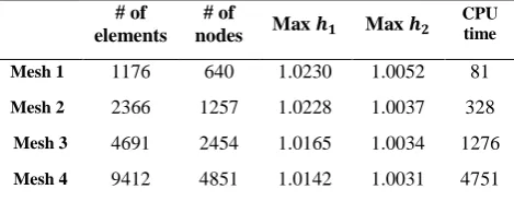
statistics of these meshes are listed in Table 1. Note that moving from the coarse mesh to the next fine mesh the number of elements and nodes are roughly doubled.

Table 1. Performance of the DG scheme for the lock-exchange problem on a flat bottom using four meshes and

N = 3. The CPU times are given in seconds

# of elements

# of

nodes Max 𝒉𝟏 Max 𝒉𝟐

CPU time

Mesh 1 1176 640 1.0230 1.0052 81 Mesh 2 2366 1257 1.0228 1.0037 328

Mesh 3 4691 2454 1.0165 1.0034 1276 Mesh 4 9412 4851 1.0142 1.0031 4751

Fig 1: The meshes used for the lock-exchange problem on a flat bottom.

Fig 3: Cross section of the water interface for the lock- exchange problem on a flat bottom at the location y = 0.5

and time t = 0.75.

4.2

Lock-exchange problem on a non-flat

bottom

We consider a test example of lock-exchange hydraulics over a hump. This problem is inspired by the works of [12, 26, 5] where tidal and exchange flow in the Strait of Gibraltar was studied using the two-layer shallow water equations. Here, the two-layer shallow water equations (1)-(2) are solved over a

bottom topography considered to be a Gaussian-shaped function defined as

𝐵 𝑥, 𝑦 = exp −𝑥2 _{. (28)}

The two layers are initially separated and the lighter water is on the left while the heavier one is on the right i.e.,

ℎ1 𝑥, 𝑦, 0 =

2 − 𝐵 𝑥, 𝑦 , if 𝑥 ≤ 0,

0, elsewhere,

ℎ2 𝑥, 𝑦, 0 =

0, if 𝑥 ≤ 0,

2 − 𝐵 𝑥, 𝑦 , elsewhere,

and

𝑢1 𝑥, 𝑦, 0 = 𝑣1 𝑥, 𝑦, 0 = 𝑢2 𝑥, 𝑦, 0 = 𝑣2 𝑥, 𝑦, 0 = 0,

The computational domain is [−3, 3] × [0, 1] and the boun-dary conditions at the downstream and the upstream of the channel are imposed on the water discharges 𝑞1 =

(𝑞1,𝑥, 𝑞1,𝑦)𝑇 and 𝑞2 = (𝑞2,𝑥, 𝑞2,𝑦)𝑇 as 𝑞1 𝛾 + 𝑞2 𝛾 ∙ 𝐧 𝛾 𝑑𝛾 = 0,

Γ

(29)

where Γ refers to the open boundaries of the channel located at

𝑥 = −3 and 𝑥 = 3, compare [26] for more details on the description of this test example.

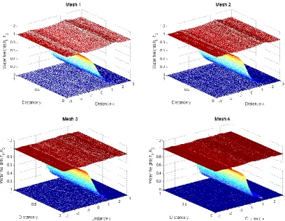
Fig 5: The mesh used for the lock-exchange problem on a non-flat bottom.

Fig 6: Cross section of the water interface for the lock-ex-change problem on a non-flat bottom at the location y =

0.5

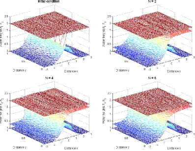
The density ratio is 𝜌1 𝜌2= 0.98 and it is expected that the heavier water propagates to the upstream, while the lighter one moves to the downstream. The solution is also expected to converge to a smooth steady state. The purpose of this example is to verify the response of the DG method for the variation of the order of polynomial approximation N. To this end the computational domain is discretized into 914 elements and the polynomial degree N is set to 2, 4 and 6. Only steady-state solutions are presented for this test example. In Figure 4 we present the steady-state numerical results for the water free-surface and the water interface using the selected orders of polynomial approximation. In this figure, we have also included the initial conditions along with the bottom bed. The water free-surface creates a strong interaction with the hump, resulting in the formation of strong and weak shocks. By using different values of N, high resolution is clearly obtained in those regions where the gradients of the water depth are steep such as the moving fronts. Apparently, the overall flow pattern for this example is preserved with no spurious oscillations appearing in the results by DG method using fixed meshes. Obviously, the obtained results verify the stability and the shock capturing properties of the proposed DG

method. In addition the proposed DG method performs well for this test problem since it does not diffuse the moving fronts and no spurious oscillations have been observed when the water flows over the hump.

Table 2. Performance of the DG scheme for the lock-exchange problem on a non-flat bottom using different polynomial degrees and a mesh of 914 elements. The CPU times are given in seconds.

Max 𝒉𝟏 Max 𝒉𝟐 CPU time

𝑵 = 𝟐 1.7060 1.727 1223

𝑵 = 𝟒 1.7296 1.775 4228

𝑵 = 𝟔 1.7483 1.802 10729

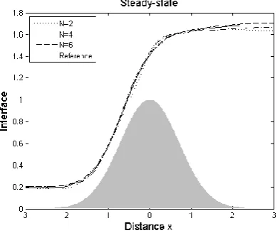
For comparison reasons, cross sections of the water interface at the channel location 𝑦 = 0.5 are shown in Figure 6 in which we have included a reference solution [22]. These results are very similar to the ones obtained in [12, 5]. It should be stressed that no interface instabilities have been observed in this example, even though initially ℎ1 = 0 for

𝑥 > 0 and ℎ2 = 0 for 𝑥 < 0 and at small times, either ℎ1 or ℎ2 is (almost) zero in a significant part of the computational domain. One of the key stability factors here is the ability of our DG method to preserve the positivity of each layer depth. For further comparisons we summarize in Table 2 the maximum values of the water heights ℎ1 and ℎ2 along with the corresponding CPU times for the three different orders 𝑁 = 2, 4 and 6. It is clear that the considered orders of polynomial approximation give roughly the same maximum values for both water heights. However, in terms of efficiency, the proposed DG method using N = 6 requires two to three times more computational work than the DG method using 𝑁 = 4.

5.

CONCLUSIONS

viscous coupling a wave model component into the modelling system to include the effects of bottom friction, wind stress, eddy viscosity, and Coriolis force in the hydraulics.

6.

ACKNOWLEDGMENTS

Financial support provided by MULIT and MHYCOF projects is gratefully acknowledged.

7.

REFERENCES

[1] R. Abgrall, S. Karni, Two-layer shallow water systems: a relaxation approach, SIAM J. Sci. Comput. 31 (2009) 1603–1627.

[2] V. Aizinger, C. Dawson, A discontinuous Galerkin method for two-dimensional flow and transport in shallow water, Advances in Water Resources 25 (2002) 67–84.

[3] Y. Bazilevs, T. Hughes, Weak imposition of Dirichlet boundary conditions in fluid mechanics, Computers & Fluids, in press 36 (2007) 12–26.

[4] F. Bouchut, T. Morales, An entropy satisfying scheme for two-layer shallow water equations with uncoupled treatment, M2AN Math. Model. Numer. Anal. 42 (2008) 683–698.

[5] M. Castro, J. García -Rodriguez, J. González -Vida, J. Macias, C. Parés, M. Vázquez-Cendón, Numerical simulation of two-layer shallow water flows through channels with irregular geometry, J. Comp. Physics. 195 (2004) 202–235.

[6] B. Cockburn, G.E. Karniadakis, C.W.S. (eds.), Discontinuous Galerkin methods. Theory, computation and applications, Lecture Notes in Computational Science and Engineering, 11. Springer-Verlag, Berlin, 2000.

[7] B. Cockburn, C. Shu, The Runge-Kutta discontinuous Galerkin method for conservation laws V: Multi-dimensional systems, J. Comput. Phys. 141 (1998) 199– 224.

[8] B. Cockburn, C.W. Shu, The Runge-Kutta discontinuous Galerkin methods for convection-dominated problems, Journal of Scientific Computing. 16 (2001) 173–261. [9] M. Dubiner, Spectral methods on triangles and other

domains, Journal of Scientific Computing 6 (1991) 345– 390.

[10]M. Dudzinski, M. Medvidova, Well-balanced path-consistent finite volume EG schemes for the two-layer shallow water equations, Computational Science and High Performance Computing. IV (2009) 121–136. [11]C. Eskilsson, S.J. Sherwin, A triangular spectral/hp

discontinuous Galerkin method for modelling 2d shallow water equations, Int. J. Numer. Methods Fluids. 45 (2004) 605–623.

[12] D. Farmer, L. Armi, Maximal two-layer exchange over a sill and through a combination of a sill and contraction with barotropic flow, J. Fluid Mech. 164 (1986) 53–76. [13] T.W. F.X. Giraldo, A nodal triangle-based spectral

element method for the shallow water equations on the sphere, Journal of Computational Physics 207 (2005) 129–150.

[14]F.X. Giraldo, T. Warburton, A high-order triangular discontinuous Galerkin oceanic shallow water model, Int. J. Numer. Meth. Fluids 56 (2008) 899–925.

[15]J. Hesthaven, From electrostatics to almost optimal nodal sets for polynomial interpolation in a simplex, SIAM J. Numer. Anal. 35 (1998) 655–676.

[16]J. Hesthaven, T.Warburton, High-order nodal methods on unstructured grids. I. Time-domain solution of maxwells equations, J Comp Phys 181(1) (2002) 186– 221.

[17]T. Hughes, G. Scovazzi, P. Bochev, A. Buffa, A multiscale discontinuous Galerkin method with the computational structure of a continuous Galerkin method, Computer Methods in Applied Mechanics and Engineering 195 (2006) 2761–2787.

[18]C.W.S. J. Qiu, B. C. Khoo, A numerical study for the performance of the Runge-Kutta discontinuous Galerkin method based on different numerical fluxes, J. Comput. Phys. 212 (2006) 540–565.

[19]S.G. J.S. Hesthaven, D. Gottlieb, Spectral Methods for Time-Dependent Problems, Cambridge University Press, Cambridge, 2006.

[20]T. Koornwinder, Two-variable analogues of the classical orthogonal polynomials, in: R.A. Askey (Ed.), Theory and Applications of Special Functions, Academic Press, San Diego, 1975.

[21]E. Kubatko, J. Westerink, C. Dawson, A. Buffa, hp discontinuous Galerkin methods for advection dominated problems in shallow water flow, Computer Methods in Applied Mechanics and Engineering 196 (2006) 437– 451.

[22]A. Kurganov, G. Petrova, Central-upwind schemes for two-layer shallow water equations, SIAM J. Sci. Comput. 31 (2009) 1742–1773.

[23]W. Lee, A. Borthwick, P. Taylor, A fast adaptive quadtree scheme for a two-layer shallow water model, J. Comp. Physics. 230 (2011) 4848–4870.

[24]R. Leveque, Finite Volume Methods for Hyperbolic Problems, Cambridge University Press, Cambridge, 2002.

[25]R.V. M.A. Taylor, B.A. Wingate, An algorithm for computing fekete points in the triangle, SIAM J. Numer. Anal. 38 (2000) 1707–1720.

[26]J. Macías, C. Parés, M. Castro, Improvement and generalization of a finite element shallow water solver to multi-layer systems, Int. J. Num. Methods Fluids. 31 (1999) 1037–1059.

[27]J. Proriol, Sur une famille de polynomes à deux variables orthogonaux dans un triangle, C.R. Acadamic Science, Paris 257, 1957.

[28]C. Shu, Total variation diminishing time discretizations, SIAM J. Sci. Stat. Comput. 9 (1988) 1073–1084. [29]S. Tu, S. Allibadi, A slope limiting procedure in