Solution of Stochastic Non Homogeneous Linear First Order Difference Equations

(1)

http://dx.doi.org/10.4236/jmf.2014.44021

How to cite this paper: Kadry, S. and El Hami, A. (2014) Solution of Stochastic Non-Homogeneous Linear First-Order Dif-ference Equations. Journal of Mathematical Finance, 4, 245-248. http://dx.doi.org/10.4236/jmf.2014.44021

Solution of Stochastic Non-Homogeneous

Linear First-Order Difference Equations

Seifedine Kadry1*_{, Abdelkhalak El Hami}2

1_{American University of the Middle East, Egaila, Kuwait} 2_{LOFIMS Laboratory, INSA de Rouen, Rouen, France}

Email: *_{[email protected]}_,_{[email protected]}

Received 28 May 2014; revised 30 June 2014; accepted 13 July 2014

This work is licensed under the Creative Commons Attribution International License (CC BY). http://creativecommons.org/licenses/by/4.0/

Abstract

In this paper, the closed form solution of the non-homogeneous linear first-order difference equa-tion is given. The studied equaequa-tion is in the form: xn = x0 + bn, where the initial value x0 and b, are

random variables.

Keywords

Stochastic Linear Difference Equations, Random Variables, Closed Form Solution, Direct Transformation Technique

1. Introduction

A difference equation or dynamical system describes the evolution of some variable over time. The value of this variable in period t is denoted by xn. The time index n takes on discrete values and typically runs over all integer

numbers Z, e.g. t = ⋅⋅⋅, −2, −1, 0, 1, 2,⋅⋅⋅. By interpreting t as the time index, we have automatically introduced the notion of past, present and future [1].

Many problems in Probability give rise to difference equations. Difference equations relate to differential eq-uations as discrete mathematics relates to continuous mathematics. Anyone who has made a study of differential equations will know that even supposedly elementary examples can be hard to solve. By contrast, elementary difference equations are relatively easy to deal with.

Aside from Probability, Computer Scientists take an interest in difference equations for a number of reasons. For example, difference equations frequently arise while determining the cost of an algorithm in big-O notation

[2]. In engineering, difference equations arise in control engineering, digital signal processing, electrical net-works, etc. In social sciences, difference equations arise to study the national income of a country and then its

*

(2)

S. Kadry, A. El Hami

246

variation with time, Cobweb phenomenon in economics [3], etc. Similar to differential equation, difference equ-ation is the most powerful instrument for the treatment of discrete processes.

Stochastic difference equations are difference equations with random parameters. Such equations arise in various disciplines, for example economics [4], physics, nuclear technology, biology and sociology. In this pa-per, we present a new technique based on the direct transformation technique to express analytically the proba-bility density function of the general solution of stochastic linear 1st order difference equations.

2. Linear 1st Order Difference Equations

A typical linear non-homogeneous first order difference equation is given by:

1 , 0 , 0

n n n n

x =a x− +b x =α n≥ (1)

where an ≠0, an and bn are real-valued functions. The unique solution of (1) may be found as follows:

(

)

1 1 0 1

2 2 1 2 2 1 0 1 2 2 1 0 2 1 2

x a x b

x a x b a a x b b a a x a b b

= +

= + = + + = + +

Now by induction, we can show:

1 1 1

0 0

0 1

n n n

n i i r

r

i i r

x a x a b

− − − = = = +   = + _ _  

∑

∏

(2)

To establish this, assume that (2) holds for order n. Then from (1) xn+1=an+1xn+bn+1, hence (2) gives:

1 1 1

1 1 0 1 0

0 0

0 1 0 1

n n n n n n

n n i i r n i i r

r r

i i r i i r

x a a x a b b a x a b

− − − + + + = = = = + = = +       = _ + _ _ _+ = + _ _     

∏

∑

∏



∏

∑

∏

Thus (2) holds for all n≥0.

There is a special case of (1) that is important in many engineering and business applications, is given by:

0 n

x =x +bn (3) This case is studied throughout this paper where x0 and b, are random variables.

3. Direct Transformation Technique

There are several versions of the Direct Transformation Technique in the literature [5]-[9]; we will provide a simple one for 1-dimension variable then for N-dimension variables.

1-dimension variable

Let X be a continuous random variable with probability density function (pdf), fX

( )

x and defined over an

interval I. Let g: I→R be a continuous one-to-one function, i.e. its inverse h: J→I

(

J⊂R

)

. Let Y = g(X), then the probability density function of Y, fY

( )

y is given by:

( )

(

1

( )

)

dd 1

( )

, for

0 otherwise

X Y

f g y g y y J

f y y

− −  × ∈  =    (4)

Example: X has probability density function given by fX

( )

x

xβ α

= (where x, α, and β are strictly positive real numbers). Let Y = −2ex, we want to find the probability density function of Y, fY

( )

y . Here

*

I=R₊,

*

J=R₋. Using (4), we have:

(3)

N-dimension variables

Let

(

X X1, 2,,Xn

)

n continuous random variable with given joint probability density function

(

)

1 2 n 1, 2, ,

X X X n

f _ x x  x . Consider a one-to-one transformation function g R: n →Rn where

(

Y Y1, 2,,Yn

)

=g X X

(

1, 2,,Xn

)

is continuous with respect to every variable and its partial derivatives is

con-tinuous as well. Then the joint probability density function of

(

Y Y1, 2,,Yn

)

is given by:

(

)

(

)

1 2 1 2

1

1 1

1

1 2 1 2

1

, , , , , ,

n n

n

Y Y Y n X X X n

n

n n

x x

y y

f y y y f g y y y

x x y y − ∂ ∂ ∂ ∂ = ∂ ∂ ∂ ∂          . (5)

4. Application

In this section, we will solve the stochastic difference equation xn=x0+bn (given in (3)), where x0 and b

are random variables with the known joint probability density function, by finding the probability density func-tion of xn using (5). So in this stochastic difference equation we have two random variables (x0, b) as input

and one random variable

( )

xn as output. For example, let

(

)

0

0, e , 0 0, 0

x b

f x b = − − x ≥ b≥ . By using (5), let

1 0

y =x and y2 =x0+bn with inverse x0= y1 and

2 1

y y

b n −

= . The joint probability density function of

1

y and y2 (Figure 1) is given by:

(

)

2 1

1

1 2 0

2 1

, 1 2 , 1

1 0

1

, , ₁ ₁ e

y y y

n

Y Y X B

y y

f y y f y

n n n n − − − −   = _ _ − = × .

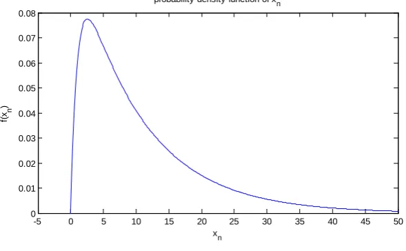
Now to find the probability density function of xn, i.e. y2 we must find the marginal probability density

function of Y2 (Figure 2) by integrating out of Y1:

(

)

2 1 2

1

2 ₂

2 2 0 1

1 1

e d e e

1

y y y

y

y _y

n n

Y n

f y x y

[image:3.595.162.461.442.709.2]

n n − − −  ₋ −  = = × =  −  −  

∫

Figure 1. Joint probability density function of y1 and y2.

0 2 4 6 8 10 0 5 10 0 0.02 0.04 0.06 0.08 0.1 y 1

Joint probability density function

y₂

f(y

1

,y 2

(4)

S. Kadry, A. El Hami

[image:4.595.167.462.90.272.2]

248

Figure 2. Probability density function of xn.

We can show easily that ₀ f y

( )

2 dy2 1

∞

=

∫

.

References

[1] Elaydi, S. (2004) An Introduction to Diﬀerence Equations. 3rd Edition, Springer-Verlag, New York. [2] King, F. (2005) Difference Equations [PDF Document]. Retrieved from Lecture Notes Online Web Site:

http://www.cl.cam.ac.uk/teaching/2004/Probability/

[3] Chui, C.K. and Chen, G. (1987) Kalman Filtering with Real-Time Applications. 2nd Edition, Springer-Verlag, New York. http://dx.doi.org/10.1007/978-3-662-02508-6

[4] Novak, S.Y. (2011) Extreme Value Methods with Applications to Finance. Chapman & Hall/CRC Press, London. http://dx.doi.org/10.1201/b11537

[5] Soong, T.T. (1973) Random Differential Equations in Science and Engineering. Academic Press, New York.

[6] Kadry, S.A. (2007) Solution of Linear Stochastic Differential Equation. USA: WSEAS Transactions on Mathematics, April 2007, 618.

[7] Kadry, S. (2012) Exact Solution of the Stochastic System of Difference Equations. Journal of Mathematical Control Science and Applications (JMCSA), 5, 67-70.

[8] Kadry, S. and Younes, R. (2005) Étude Probabiliste d’un Système Mécanique à Paramètres Incertains par une Tech-nique Basée sur la Méthode de transformation. Proceedings of the 20th Canadian Congress of Applied Mechanics (CANCAM’ 05), Montreal, 30 May, 490-491.

[9] Kadry, S. (2012) Probabilistic Solution of Rational Difference Equations System with Random Parameters. ISRN Ap-plied Mathematics, 2012, Article ID: 290186. http://dx.doi.org/10.5402/2012/290186

-5 0 5 10 15 20 25 30 35 40 45 50

0 0.01 0.02 0.03 0.04 0.05 0.06 0.07 0.08

x_n

f(x

n

)

(5)