Mining Attributes Patterns of Defective Modules for
Object Oriented Software
Bharavi Mishra
Dept. Computer Engineering. Indian Institute of Technology
(BHU), Varanasi, 221005
K.K. Shukla
Dept. Computer Engineering. Indian Institute of Technology (BHU), Varanasi, 221005
ABSTRACT
Defect prediction is the process of predicting the fault prone module using some pre-mined patterns or rules. Several statistical and mathematical strategies have been used in recent past to mine these rules. However, the interpretability of these rules is the matter of concern. In real development process an expert is required to demonstrate the working of mined patterns which prevents the use of these mined patterns in software development process. Considering these facts, in this study we tried to find the combination of attribute-value pair which indicates the bug. These attribute-value pair is known as defect pattern. For defect pattern mining we used GUHA (General Unary Hypothesis Automaton) procedure which is oldest yet very powerful method of pattern mining. The basic idea of GUHA procedure is to mine the entire possible and interesting hypothesis supported by the data in predefined logical form. The experimental results show that the mined patterns can be used as a rule to identify the defective module. Moreover, the mined patterns do not suffer from the interpretability problems.
Keywords
Defect patterns, GUHA, Fault prediction.
1.
INTRODUCTION
With the increasing demand of multipurpose software today, the constraints and complexity involved with the development of software are rising. The multiple and accurate functionality that the software are required to meet, pose a high level of fault proneness within the structure of software model. Developing software without fault is still a challenging task for software engineers. Fault prone software incurs a large cost in terms of both time and effort. One of the ways to reduce the development cost is the prediction of some important software quality attributes like reliability, testability, fault proneness, effort estimation and maintainability in the preliminary stage of software development. A software fault prediction is well known and proven technique to produce high quality software. The availability of public data repository [1] and public domain models [2] can ease the task of model generation and test. In literature several statistical and machine learning techniques have been applied to develop defect prediction model. Neural networks have been used [5] in software metrics such as such as object-oriented metrics to predict the defect proneness of software module and to evaluate the quality of software products. The defect proneness of software modules can also be investigated using the regression technique. Bibi et al.[7] and Graves et al.[8] applied the regression techniques on the change history of software products in order to accurately predict defect proneness of software modules. Salemet et al. [9] applied the regression on the test cases to estimate the
number of defects that can be detected. The clustering can be applied on the data specified by experts according to complexity metrics of software products to cluster the fault prone modules and not fault prone modules [10]. Menzis et al [3] carried out a comparative study using Naive Bayes [18], Oner [16] and J48 [17] classification models on static code attribute data sets to evaluate the application of these models in defect prediction.
Although the aforementioned techniques such as NN, regression and clustering have been used successfully in software defect prediction ,however, most of them suffers from Interpretability problem because they work as a black box and requires experts while applying in software industries. On the other hand rule based classifiers suffers from two basic problems First, classification mining is used to obtain the minimum set of rules. Second, the imbalance data set needs additional processing, such as under-sampling or oversampling, when constructing decision trees. Therefore, we can use other data mining techniques such as association rule mining technique to find all the rules with a higher level of support and confidence, and can be utilized to describe the relationship between attributes of software modules and defects [15]. The main advantage of using association rule mining is that the mined patterns set can be used to describe software defect behaviours. To facilitate the description of defect behaviours, this study defines defects patterns as a set of values of attributes that can be used to describe and predict the occurrence of defects. The defect patterns of products consisting of set of attribute–value pair which tends to bug. To determine whether a product contains defects, the attributes of the products are compared with defect patterns. GUHA is a method of exploring data analysis. It can be used as an alternative method for association rule mining. It has been used successfully in medical diagnosis and financial data analysis. GUHA mines all the hypothesis of the form A S from the data set based on associated quantifiers where A and S are the set of attributes. GUHA uses the bit string method for exploring the hypothesis. The objective of this paper is to evaluate the application of GUHA in software defect prediction. To mine all the defect patterns we apply GUHA on KC1 data set to mine all the patterns of the form A S where A is the set of attribute-value pair and S is the class attribute whose value is buggy.
The rest of the paper is organized as follows. Section 2 presents the overview of bug database. Thereafter, in section 3 Introduction of association rule mining and GUHA procedure are presented. Experimental set-up is given in section 4. Result and discussion is presented in section 5. Section 6 concludes the paper and provides the future direction.
2.
DATA SET
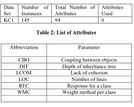
KC1 is the storage management software for receiving and processing the ground data.KC1 is the object oriented software written in C++ language. KC1 defect data set contains the information regarding class level attributes. It has over all 145 instances with 94 attributes. These attributes are classified into two groups. First group, group A contains 10 attributes whereas second group, group B has overall 84 attributes. In the present study we used 6 most widely used object oriented attributes [13] from set A because all the group B attributes are measured on method level and latter transformed into the module level attributes. Information regarding data set and attributes are given in table 1 and table 2.
Table 1: KC1 Data Set
Data Set
Number of Instances
Total Number of Attributes
Attributes Used
[image:2.595.56.280.231.410.2]KC1 145 94 6
Table 2: List of Attributes
Abbreviation Parameter
CBO Coupling between objects DIT Depth of inheritance tree LCOM Lack of cohesion
LOC Number of lines RFC Response for a class WMC Weight method per class
3.
ASSOCIATION RULE MINING
An association rule is a probability based statement of co-occurrence of certain items. Association rule mining is a process of discovering the relationships between seemingly unrelated data in transaction database or other data repositories. An association rule is commonly represented using the notation X Y which means the transaction database containing the item set X tend to contain the item set Y. Two measurement thresholds support and confidence, measures the intensity of the generated association rule. More formally, for a given transaction T={ T1,T2…….Tn),where each transaction Ti is the set of items, I ={ I1,I2,…..Im).
An association rule is described as A B where A I, B I and A B = with Support=Sup and Confidence =Con where Support , and Confidence defined as
Sup=
Con=
An association rule mining task is to find all the association rules of the form X Y such that the support and confidence of all the association rules are above the user defined support and confidence. A traditional association rule mining task does not have any predefined target. It means that it does not have any predefined antecedents and consequents. The traditional association rule mining algorithm, A-priori [11],
Step 2. In second step, it generates all the association rules with the confidence at least user
specified confidence.
In association rule mining an item can be represented using the Boolean representation. It is a category based representation of the transaction database. In this way a Boolean data matrix is generated using the whole transaction database. Each row of data matrix corresponds to one observed object; each column corresponds to one attribute. Each attribute has finite number of possible values called categories. Thus these attributes are called categorial attributes. In this representation each attribute of transaction database is transformed into the Boolean data matrix based on the finite number of possible values contained by that attribute. Bit string representation [12] is based on cards of categories. The card of category is a string of bits. For example if an attribute A has five distinct values {1,2,3,4,5} under its belt, it is transformed into five different columns of Boolean data matrix where each value of attribute A is denoted as A[x] where x is the available category. It also means that the attribute A is represented by card A[1]……A[5] for category 1…5.Therefore, each column of the resultant data matrix M corresponds to one value of attribute A (Table 3). In Boolean data matrix value “1” in ith
row and A[x]th column indicates that ith instance has A[x]th attribute value.
[image:2.595.321.535.453.566.2]This bit string approach facilitated us to mine not only the association rules based on support and confidence threshold but also various additional relation of Boolean attribute including statistical hypothesis. The bit string approach provides the basics of GUHA procedure. Next we will explain the GUHA procedure.
Table 3: Bit String Based Transformation of Attribute.
Original Data
Transformed Data or Cards of Attribute A
Row A A[1] A[2] A[3] A[4] A[5]
R1 1 1 0 0 0 0
R2 5 0 0 0 0 1
R3 4 0 0 0 1 0
R4 3 0 0 1 0 0
. . . .
. . . .
Rn 2 0 1 0 0 0
3.1
GUHA
The hypothesis generated by GUHA procedure shows that most of the generated objects satisfying the antecedent satisfy the succedent also. Moreover, the number of objects satisfying the antecedent should be greater than the predefined threshold. It is stressed that the found results are formulas true in the data and they are hypothesisfrom the point of view of the data. In other words we can say “GUHA offers everything interesting”[12].
The procedure 4FT miner mines all the hypothesis of the form A ≈ S where A and S are the set of categorical attributes which are connected with the Boolean connectives. The generated association rules are verified using the Boolean data matrix M. Each pair of (A,S) produces a four-fold table (table 4). The association rule A ≈ S is true in the concerning data matrix if the condition corresponding to the used quantifier such as founded implication, is satisfied in the four-fold table (fft) which is also known as contingency table of cedents in M [12].
The fft , Table 4, in data matrix is the quadruple (a,b,c,d) of natural numbers which contains the information of satisfiability of a particular hypothesis in the data matrix derived from the quantifier used for generation. These natural numbers indicates
a is the number of rows satisfying cedents and can be expressed as Count(Card(A) Card(S))
b is the number of rows satisfying A but not S and can be expressed as Count(Card(A)-a)
c is the number of rows satisfying S but not A and can be expressed as Count( Card(S)-a)
d is the number of rows not satisfying cedents and can be expressed as n-a-b-c, where n is the number of instances in the data matrix.
As discussed earlier, the Card of the Boolean attributes is a string of bits that is analogous to the card of the category and is used to count the frequency of the attributes in the data matrix.
Table 4: 4 FT table
M S ~S A a b ~A c d
4 FT GUHA procedure has various different types of quantifiers that can be used to mine association rules which have different types of relations between cedents. In this study our basic aim is to mine all the patterns of attributes related with the buggy class. Therefore, we use basic 4FT quantifier “founded implication” for defect pattern mining.
Founded Implication is denoted as p, Base . This quantifiers
has two parameters p and Base such that p≤ 1 and Base > 0 with the constraint The association rule A p, Base S shows that at least 100p percent of rows of data
matrix M satisfying A also satisfy S where at least Base rows
of M satisfy both A and S. GUHA procedure for association rule mining is shown in figure 1.
Input:- Transformed Boolean Data Matrix Output:- Set of Relevant Association rules
Generate all Relevant Antecedents For each Antecedent
If Count(Card(Antecedent)) < Base Next Antecedent
Else
Generate all Relevant Succedents For each Succedent
Generate Association Rule A_R with (Antecedent,
Succedent)
If A_R is a true association rule Add A_R to final rule set. Else
Next Succedent Endfor
Endfor
Figure 1: Pseudo code for 4 ft GUHA procedure[12]
4.
EXPERIMENTAL SET-UP
The objective of this section is to describe the experimental set-up used in this study. In this section first the goal of our study is presented. Thereafter, transformation of data into the bit string format is described. We used the open source Lisp-miner [19] machine learning toolkit to conduct this study. GUHA 4 FT miner is implemented in Lisp-miner toolkit.
4.1. GOAL
The goal of our study is to mine all the attribute based defect patterns that lead to buggy module or class.
4.2
BIT STRING TRANSFORMATION
OF DATA
There are six independent attributes based on the metric induced by Object Oriented design [13] and one dependent attribute class. Each of the attributes need to transformed into the bit string format before applying the 4 FT procedure of GUHA. The result of attribute transformation is listed in table 5. Attributes CBO, DIT, LCOM, RFC, class and WMC are transformed using “each value one category transformation”. It means that each distinct value of the attribute is treated as a single category. In attribute LOC there are approximately 144 distinct values so after transformation it poses 144 categories. Therefore, we used interval transformation for attribute LOC. The transformed Boolean data set has 195 categorical attributes and 144 instances.
4.3
PARAMETER TUNING
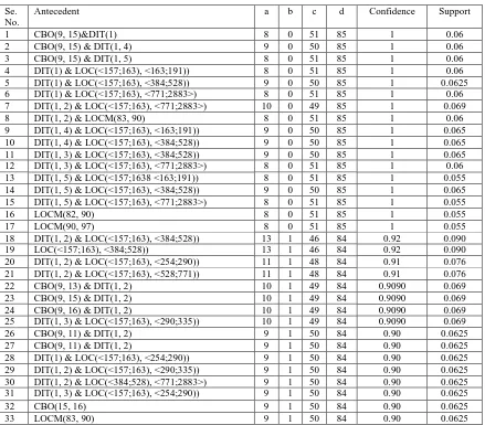
Table 6. List of Generated Hypothesis
Se. No.
Antecedent a b c d Confidence Support
1 CBO(9, 15)&DIT(1) 8 0 51 85 1 0.06
2 CBO(9, 15) & DIT(1, 4) 9 0 50 85 1 0.06
3 CBO(9, 15) & DIT(1, 5) 8 0 51 85 1 0.06
4 DIT(1) & LOC(<157;163), <163;191)) 8 0 51 85 1 0.06 5 DIT(1) & LOC(<157;163), <384;528)) 9 0 50 85 1 0.0625 6 DIT(1) & LOC(<157;163), <771;2883>) 8 0 51 85 1 0.06 7 DIT(1, 2) & LOC(<157;163), <771;2883>) 10 0 49 85 1 0.069
8 DIT(1, 2) & LOCM(83, 90) 8 0 51 85 1 0.06
9 DIT(1, 4) & LOC(<157;163), <163;191)) 9 0 50 85 1 0.065 10 DIT(1, 4) & LOC(<157;163), <384;528)) 9 0 50 85 1 0.065 11 DIT(1, 3) & LOC(<157;163), <384;528)) 9 0 50 85 1 0.065 12 DIT(1, 3) & LOC(<157;163), <771;2883>) 8 0 51 85 1 0.06 13 DIT(1, 5) & LOC(<157;1638 <163;191)) 8 0 51 85 1 0.055 14 DIT(1, 5) & LOC(<157;163), <384;528)) 9 0 50 85 1 0.065 15 DIT(1, 5) & LOC(<157;163), <771;2883>) 8 0 51 85 1 0.055
16 LOCM(82, 90) 8 0 51 85 1 0.055
17 LOCM(90, 97) 8 0 51 85 1 0.055
18 DIT(1, 2) & LOC(<157;163), <384;528)) 13 1 46 84 0.92 0.090 19 LOC(<157;163), <384;528)) 13 1 46 84 0.92 0.090 20 DIT(1, 2) & LOC(<157;163), <254;290)) 11 1 48 84 0.91 0.076 21 DIT(1, 2) & LOC(<157;163), <528;771)) 11 1 48 84 0.91 0.076 22 CBO(9, 13) & DIT(1, 2) 10 1 49 84 0.9090 0.069 23 CBO(9, 15) & DIT(1, 2) 10 1 49 84 0.9090 0.069 24 CBO(9, 16) & DIT(1, 2) 10 1 49 84 0.9090 0.069 25 DIT(1, 3) & LOC(<157;163), <290;335)) 10 1 49 84 0.9090 0.069 26 CBO(9, 11) & DIT(1, 2) 9 1 50 84 0.90 0.0625 27 CBO(9, 11) & DIT(1, 2) 9 1 50 84 0.90 0.0625 28 DIT(1) & LOC(<157;163), <254;290)) 9 1 50 84 0.90 0.0625 29 DIT(1, 2) & LOC(<157;163), <290;335)) 9 1 50 84 0.90 0.0625 30 DIT(1, 2) & LOC(<384;528), <771;2883>) 9 1 50 84 0.90 0.0625 31 DIT(1, 3) & LOC(<157;163), <254;290)) 9 1 50 84 0.90 0.0625
32 CBO(15, 16) 9 1 50 84 0.90 0.0625
33 LOCM(83, 90) 9 1 50 84 0.90 0.0625
Table: 5 Attribute Categorization.
Attribute Transformation Type Number of categories CBO Each Value One Category
Transformation
25
DIT Each Value One Category Transformation
5
LCOM Each Value One Category Transformation
41
Class Each Value One Category Transformation
2
RFC Each Value One Category Transformation
63
WMC Each Value One Category Transformation
39
LOC Interval Transformation 20
5.
RESULT AND DISCUSSION
The results of our experiments are shown in table 6. Each row of the table contains the generated hypothesis, their respective
defect patterns is to reduce testing costs and increase the quality, by distributing the testing efforts to only fault-prone classes, since to test each and every module is infeasible. The patterns generated by GUHA procedure are very simple and intuitive. This helps the developers to establish hypothetical Section 3 and subsection 3.1), use no additional space above the subsection head. relationships between object oriented metrics and fault prone classes which ease the task of class selection for testing. In such strategy, a programmer is mainly interested in the correct detection of faulty classes. Observing the results, we can conclude that CBO value > 9 and higher value of LCOM are related to the presence of a fault in the class. CBO value > 9 associated with different value of DIT are related with the buggy modules., In other rules, The classes with LOC value > 163 associated with different value of DIT are more bug prone. There is no rule related to the metric WMC and RFC with higher confidence, therefore not reported in the list. The patterns presented here indicate the classes with higher likelihood of being faulty; therefore the classes with these features need more attention during testing. On the other hand, we can also use these patterns after the design phase and during the coding phase of software development in integrated manner. We can build a spin-lock type system which consists of these patterns in the form of IF THAN ELSE rules and attribute measurement modules. This system continuously measures the value of different attributes and warns the programmer if the module cross the danger threshold of attribute value.
6.
CONCLUSION
AND
FUTURE
DIRECTION
This paper empirically evaluates the application of GUHA in software defect prediction. On base of experimental results we concludes that GUHA is the suitable tool for discovering unrevealed information or patterns from the bug database which is not possible using traditional black box models. It generates more understandable and precise results which can help in real development process to produce quality software. In addition, in the view of on KC1 database, experimental results also reveal that attributes CBO, DIT, LCOM, and LOC are more likely related with bug. Attribute-value pair combination, listed in table 6, can be used to identify the buggy class.
In future we plan to extend our study on more bug datasets. In this study our main objective is to find the patterns for buggy class in future we plan to find the attributes patterns for bug proneness. GUHA procedure generates very large number of patterns which are very tricky to handle. Therefore, we also plan to use some rule subset selection techniques to find more precise and suitable patterns or rules.
7.
REFERENCES
[1]. Promise. http://promisedata.org/repository/.
[2]. Weka. http: //www.cs.waikato.ac.nz /.
[3]. Menzies, T., Dekhtyar, A., Distefano, J., and Greenwald, J. 2007. Problems with Precision: A Response to Comments on Data Mining Static Code Attributes to
Learn Defect Predictors. IEEE Trans. Software Eng., vol. 33, no. 9,pp. 637-640, Sept.
[4]. Zhong, S., Khoshgoftaar, T.M., Seliya, N. 2002. Analyzing software measurement data with clustering techniques, IEEE Intelligent System 19 20–27.
[5]. Thwin, M.M., Quah, T.S. 2005. Application of neural networks for software quality prediction using object-oriented metrics, The Journal of Systems and Software 76 147–156.
[6]. Khoshgoftaar, T.M., Lanning, D.L. 1995. A neural network approach for early detection of program modules having high risk in the maintenance phase, Journal of Systems and Software 29 (1) 85–91.
[7]. Bibi, S., Tsoumakas, G., Stamelos, I., Vlahavas, I. 2008. Regression via classification applied on software defect estimation, Expert Systems with Applications 34 2091– 2101.
[8]. Graves, T., Karr, J.A., Marron, H.S. 2000. Predicting fault incidence using software change history, IEEE Transactions on Software Engineering 26 (7) 653– 661.
[9]. Salem, A.M., Rekabb, K., Whittakerc, J.A. 2004. Prediction of software failures through logistic regression, Information and Software Technology 46 519–523.
[10].Hand, D., Mannila, H., Smyth, P. 2001. Principles of Data Mining, MIT Press, Cambridge, MA.
[11].Agrawal, R., Srikant, R. 1994. Fast algorithm for mining association rules, Proceeding of the 20th VLDB conference, Morgan Kaufmann, Santiago, Chile, pp. 487– 499.
[12].Hajek, P., Holeˇna, M., Raucha, J., 2010. The GUHA method and its meaning for data miningJournal of Computer and System Sciences 76 34–48
[13].Chidamber, S.R., Kemerer, C.F., 1994. A metrics suite for object oriented design. IEEE Transaction on Software Engineering 20 (6), 476–493.
[14].Hajek, P., Havel, I., Chytil, M. 1996. The GUHA method of automatic hypotheses determination, Computing .
[15].Huntley, C.L. 2003. Organizational learning in open-source software projects: an analysis of debugging data, IEEE Transactions on Engineering Management 50 (4) 485–493.
[16].R. Holte, R. 1993“Very simple classification rules perform well on most commonly used datasets,” Machine Learning, vol. 11, p. 63.
[17].Quinlan, R. 1992. C4.5: Programs for Machine Learning. Morgan Kaufman.
[18].Witten I. H., and Frank, E., 2005. Data mining. 2nd edition. Los Altos, US: Morgan Kaufmann.