Video over Cellular Mobile Device based on Hybrid Technique

Video over Cellular Mobile Device based on Hybrid

Technique

1

Fouad Hammadi Awad

College of Computer - Anbar University – Anbar – Iraq

2

Muzhir

Shaban AL-Ani

College of Computer - Anbar University – Anbar – Iraq

ABSTRACT

Video compression is considered of high importance especially for mobile devices such as laptops and cellular devices. Thus the need for adapting video signal over these device arises mainly to save bandwidth and reduce time. In this paper a new method is proposed of adapting video signal over cellular mobile devices by combining an adaptive method and a compression method (JPEG). JPEG is a standardized image compression mechanism, but in this paper used a different huffman coding for our compression method instead. The compression algorithm is modified to incorporate compression 24 color image as well as 8 bit gray scale image. DCT is used for transform coding. Run-length and Huffman coding are used for achieving compression. Using this approach the 24 bit color image is compressed.

General Terms

Video over mobile, lossless and lossy compression, video adapting

Keywords

Adapting of video, video over mobile, JPEG Algorithm, video compression.

1.

INTRODUCTION

The huge usage of digital multimedia via communications, wireless communications, Internet, Intranet and cellular mobile leads to incurable growth of data flow through these Media. The researchers go deep in developing efficient techniques in these fields such as compression of data, image and video. Recently, video compression techniques and their applications in many areas (educational, agriculture, medical …) cause this field to be one of the most interested fields [1]. digital video techniques have been used for a number of years, for example in the (TV) broadcasting industry and video mobile conference . However, until recently a number of factors have prevented the wide spread use of digital video. An analog video signal typically occupies a bandwidth of a few mega hertz. However, when it is converted into digital form, at an equivalent quality, the digital version typically has a bit rate well over 100 Mbps. This bit rate is too high for most networks or processors to handle. Therefore, the digital video information has to be compressed before it can be stored or transmitted. Over the last couple of decades, digital video compression techniques have been constantly improving. Many international standards that specialize in different digital video applications have been developed or are being developed. At the same time, processor technology has improved dramatically in recent years. The availability of cheap, high-performance processors together with the development of international standards for video compression has enabled a wide range of video communications applications[2]. All video coding standards make use of the

to substantially reduce its bit rate. A still image, or a single frame within a video sequence, contains a significant amount of spatial redundancy. To eliminate some of this redundancy, the image is first transformed. The transform domain provides a more succinct way of representing the visual information. Furthermore, the human visual system is less sensitive to certain components of the transformed information. For this reason, these components can be eliminated without seriously reducing the visual quality of the decoded image. The remaining information can then be efficiently encoded using entropy encoding (for example, variable length coding such as Run-Length coding) [3].

2.

LITERATURE REVIEW

Many papers and researches are published related to this subject as below:

XueBai et al. introduced a new color model, Dynamic Color Flow, which incorporates motion estimation into color modeling in a probabilistic framework, and adaptively changes model parameters to match the local properties of the motion. The proposed model accurately and reliable describes changes in the science's appearance caused by motion across frames [4].

EugeniyBelyaev et al. proposed a new spatial scalable and low complexity video compression algorithm based on multiplication free three dimensional discrete pseudo cosine transform. This paper shows an efficient results compared with H.264/SVC as well as it can be used for robust video transmission over wireless channels [5].

EvgencyKaminsky et al., proposed an effective DCT-domain video encoder architecture that decreases the computational complexity of conventional hybrid video encoders by reducing the number of transform operations between the pixel and DCT domain. The proposed system is based on the conventional hybrid coder and on a set of fast integer composition DCT transform. The proposed architecture may be used for the future Internet and 4G applications [6]. Cong Dao Han et al., implemented a novel search algorithm which utilizes an adaptive hexagon and small diamond search to enhance search speed. Simulation results showed that the proposed approach can speed up the search process with little effect on distortion performance compared with other adaptive approaches [7].

V. Vijayalakshmi et al., proposed a new video encryption scheme for sensitive applications. The objective of the proposed system is to analyze a secure and computational feasible video encryption algorithm for MPEG video to improve the security of existing algorithm by combining encryption in Intra and Inter frames and to test the algorithm against the common attacks [8].

the most effective, will improve the compression results. Simulation results demonstrate that lower bit rates are achieved [9].

3.

MPEG TYPES

MPEG is an asymmetrical system. It takes longer to compress the video than it does to decompress it in the DVD player, PC, set-top box or digital TV set. There are many types of MPEG such as [10, 11].

3.1 MPEG-1

Although MPEG-1 supports higher resolutions, it is typically coded at 352x240 x 30fps (NTSC) or 352x288 x 25fps (PAL/SECAM). Full 704x576 and 704x480 frames (BT.601) were scaled down for encoding and scaled up for playback [16]. MPEG-1 uses the YCbCr color space with 4:2:0 sampling, but did not provide a standard way of handling interlaced video. Data rates were limited to 1.5 Mbps, but often exceeded[12].

3.2 MPEG-2

MPEG-2 provides broadcast quality video with resolutions up to 1920x1080. It supports a variety of audio/video formats, including legacy TV, HDTV and five channel surround sound. MPEG-2 uses the YCbCr color space with 4:2:0, 4:2:2 and 4:4:4 sampling and supports interlaced video.data rates are from 1.5 to 60 Mbps [12].

3.3 MPEG-4

MPEG-4 is an extremely comprehensive system for multimedia representation and distribution. Based on a variation of Apple's QuickTime file format, MPEG-4 offers a variety of compression options, including low-bandwidth formats for transmitting to wireless devices as well as high-bandwidth for studio processing. A major feature of MPEG-4 is its ability to identify and deal with separate audio and video objects in the frame, which allows separate elements to be compressed more efficiently and dealt with independently. User-controlled interactive sequences that include audio, video, text, 2D and 3D objects and animations are all part of the MPEG-4 framework[12].

3.4 MPEG-7

MPEG-7 is about describing multimedia objects and has nothing to do with compression. It provides a library of core description tools and an XML-based Description Definition Language (DDL) for extending the library with additional multimedia objects. Color, texture, shape and motion are examples of characteristics defined by MPEG-7[12].

3.5 MPEG-21

MPEG-21 provides a comprehensive framework for storing, searching, accessing and protecting the copyrights of multimedia assets. It was designed to provide a standard for digital rights management as well as interoperability. MPEG-21 uses the Digital Item as a descriptor for all multimedia objects. Like MPEG-7, it does not deal with compression methods [12].

4.

Video Formats

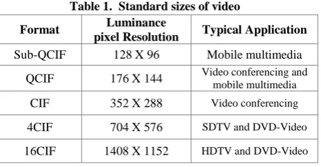
Digital video frames that are displayed at a prescribed frame rate. For example, frame rate of 30 frames/sec is used in NTSC video. The Common Intermediate Format (CIF) has 352 x 288 pixels, and the Quarter CIF (QCIF) format has 176 x 144 pixels as shown in table 1 [12].

Table 1. Standard sizes of video

5.

System Implementation of adapting

Video over mobile

The system implements two major steps that convert and compress video into its final desired form. The video is first decomposed into series of images. Then, each image is adapted to meet the target video size. The images are then sent to the compression method (JPEG) to be compressed before it goes to final video reconstruction. These steps are described below:

5.1 Adapting Video

For this step, the video is processed as a series of 24-bits still images to transform it to the target phone size. It reduces the size of the video by a measurable amount through converting every MxN pixels to a corresponding one pixel. The resulting pixel is an average of the MxN pixels. MxN is calculated through dividing the size of the image from the original video by the size of the target video. The steps below show an example of adapting 600x400 into 300x200 video:

Step1: acquiring M and N values by: M=Source video height / target video height M=600/200 = 2

N= Source video width / target video width N=400/200 = 2

Step2: converting the source video to its new size for i=0 to source video height, step M

for j=0 to source video width, step N target pixel= _𝑀𝑥𝑁1 𝑖+𝑀_𝑖 𝑗 +𝑁_𝑗 𝐼 𝑖, 𝑗

Step3: return the new sized image and call the compression method to further compress it before final video reconstruction.

5.2 Video compression based JPEG

JPEG has four modes and many options. It is more like a shopping list than a single algorithm. For our purposes, though only the lossy sequential mode is relevant, and that one is illustrated in Fig.1 Furthermore, this paper will concentrate on the way of the proposed method adapting and JPEG is normally used to encode 24-bit RGB images.

Step 1 of encoding an image with JPEG is block preparation. In order to specificity this paper assume that the JPEG input is a 640×480 RGB image with 24 bits/pixel, as shown in Fig 2(a). Since using luminance and chrominance gives better compression, must first compute the luminance Y and the two chrominances Cb, Cr and the inverse, according to the following equations1, 2 :

Y = 0.299R + 0.587G + 0.114B … . . (1) Cb = 0.564(B − Y)

Cr = 0.713(R − Y)

R = Y + 1.402Cr … … … … (2) G = Y − 0.344Cb − 0.714Cr

B = Y + 1.772Cb

Format Luminance

pixel Resolution Typical Application

Sub-QCIF 128 X 96 Mobile multimedia QCIF 176 X 144 Video conferencing and _{mobile multimedia}

CIF 352 X 288 Video conferencing

4CIF 704 X 576 SDTV and DVD-Video

Fig 1: The operation of adapting and JPEG in lossy sequential mode.

Separate matrices are built for Y, Cb , and Cr, each with elements in the range 0 to 255. Next, square blocks of four pixels are averaged in the Cb and Cr matrices to reduce them to 320×240. This reduction is lossy, but the eye barely notices it since the eye responds to luminance more than to chrominance. However, it compresses the total amount of data by a factor of two. Finally, each matrix is divided up into 8×8 blocks. The Matrix has 4800 blocks; the other two have 1200 blocks each, as shown in fig 2(b).

Fig 2: JPEG Encoding (a) RGB input data. (b) After block preparation.

Step 2 of JPEG is to apply a DCT(Discrete Cosine Transformation) according to equations 3 and 4 to each of the 7200 blocks separately. The output of each DCT is an 8×8 matrix of DCT coefficients. DCT element (0, 0) is the average value of the block. The other elements tell how much spectral power is present at each spatial frequency. In theory a DCT is lossless but in practice using floating-point numbers and transcendental functions always introduces some round off error that results in a little information loss. Normally, these elements decay rapidly with distance from the origin (0, 0) as shown in Fig 3.

Fig 3: DCT Structure (a) One block of the Y matrix. (b) the DCT coefficients.

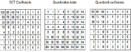
After the DCT is complete, JPEG moves on to step 3, called quantization.In which the less important DCT coefficients are wiped out. This lossy transformation is done with table quality 50 by dividing each of the coefficients in the 8×8 DCT matrix by a weight taken from a table. If all the weights are 1, the transformation does nothing

.

However, if the weights increase sharply from the origin,

higher spatial frequencies are dropped quickly. An example of this step is given in Fig 4, in which we see the

initial DCT matrix, the quantization table and the result obtained by dividing each DCT element by the corresponding quantization table element. The values in the quantization table are not part of the JPEG standard. Each application must supply its own allowing it to control the loss-compression trade-off.

Fig 4: Computation of the quantized DCT coefficients.

referred to as the DC components the other values are the AC components.

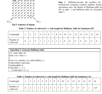
Step 5 linearizes the 64 elements and applies run-length encoding to the list. Scanning the block from left to right and then top to bottom will not concentrate the zeros together, so a zigzag scanning pattern is used as shown in Fig 5.

Fig 5: sequence of zigzag.

In this example, the zigzag pattern produces 30 consecutive 0s at the end of the matrix. This string can be reduced to a single count saying there are 30 zeros, a technique known as run-length encoding as following:

Example data: 20,17,0,0,0,0,11,0,-10,-5,0,0,1,0,0,0, 0 , 0 ,0 , only 0,..,0

RLC for JPEG compression (0,20) ; (0,17) ; (4,11) ; (1,-10) ; (0,-5) ; (2,1); EOB.

Step 6 Huffman-encodes the numbers for storage or transmission assigning common numbers shorter codes that uncommon ones.the details of Huffman table for luminance DC in table .2 and Huffman table for chrominance AC in table 3.

Table 2. Number of codeword v s. code length for Huffman table for luminance DC

Codelength 1 2 3 4 5 6 7 8 9 10 11 12 13 14 15 16

Number of

codeword 0 1 5 1 1 1 1 1 1 0 0 0 0 0 0 0

Algorithm 1: Generate Huffman table

i=0 , code value =0; for(k=1;k<=16;k++) {

For(j=1;j<=number_of_codeword[k];j++) Codeword[i]=codevalue;

Codelength[i]=k; Codevalue++; i++; { Codevalue*=2; }}

Table 3. Number of codeword vs. code length for Huffman table for luminance AC.

Codelength 1 2 3 4 5 6 7 8 9 10 11 12 13 14 15 16

Number of

codeword 0 2 1 3 3 2 4 3 5 5 4 4 0 0 1 125

6.

EXPERIMENTS AND RESULTS

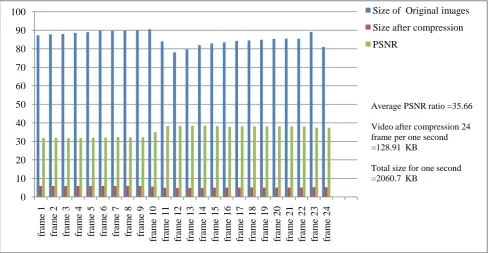
The proposed method was tested on a 24 frames per seconds video of size 2060.7 KB and the resulting compressed video was 128.9 KB and the average PSNR ratio is (35.66). The results of each frame are shown in Fig 5.

7.

CONCLUSION

Video compression is an extremely important part of modern computing by having the ability to compress videos to fraction of their original size valuable and expensive disk space can be saved. In addition, transportation of videos from one computer to another becomes easier and less time consuming (which is why image compression has played such as important role in the development of the internet). The JPEG image compression algorithm provides a very effective

Fig 5: Results and Experiments.

8.

REFERENCE

[1] Muzhir Shaban Al-Ani and Talal Ali Hammouri "Video Compression Algorithm Based on Frame Difference Approaches", International Journal on Soft Computing ( IJSC ) Vol.2, No.4, November 2011.Ding, W. and Marchionini, G. 1997 A Study on Video Browsing Strategies. Technical Report. University of Maryland at College Park.

[2] Iain E. G. Richardson ," H.264 and MPEG-4 Video – compression" , John Wiley & Sons Ltd, The Atrium, Southern Gate, Chichester West Sussex PO19 8SQ, England ,2003.

[3] Lian E. G. Richardson , " video codec design

developing image and video compression systems" , JOHN WILEY & SONS Ltd, Baffins Lane chichester ,

West Sussex PO19 IUD, England , 2002. Sannella, M. J. 1994 Constraint Satisfaction and Debugging for Interactive User Interfaces. Doctoral Thesis. UMI Order Number: UMI Order No. GAX95-09398., University of Washington.

[4] XueBai et al. "Dynamic Color Flow: A Motion Adaptive Color Model for Object Segmentation in Video", ECCV 2010, part V, LNCS 6315, pp 617-630, 2010.Brown, L. D., Hua, H., and Gao, C. 2003. A widget framework for augmented interaction in SCAPE. [5] EugeniyBelyaev et al., "Scalable Video Coding Based on

Three Dimensional Discrete Pseudo Cosine Transform", ruSMART/NEW2AN 2010, LNCS 6294, pp 448-459, 2010.Spector, A. Z. 1989. Achieving application requirements. In Distributed Systems, S. Mullender. [6] EvgencyKaminsky et al., "DCT-domain coder for Digital

Video Applications", Journal of Real Time Image Processing, 14 August 2010.

[7] Cong Dao Han et al., "An Adaptive Fast Search Algorithm for Block Motion Estimation in H.264", Journal of Zhejiang University Science C (Computer &

[8] V. Vijayalakshmi et al., "Efficient of Intra and Inter Frames in MPEG Video", CNSA 2010, CCIS 89, pp 93-104, 2010.

[9] Mohamed Haj Taieb et al., "Turbo Code Using Adaptive Puncturing for Pixel Domain Distributed Video Coding", ICISP 2010, LNCS 6134, pp 342-350, 2010.

[10]Jerome Gorin et al., "LLVM – Based and Scalable MPEG-RVC Decoder", Journal of Real Time Image Processing, 27 July 2010.

[11]V. Vijayalakshmi et al., "Efficient of Intra and Inter Frames in MPEG Video", CNSA 2010, CCIS 89, pp 93-104, 2010. (fulltext34).

[12]MPEG Definition from PC Magazine Encyclopedia http://www.pcmag.com/encyclopedia_term/0%2C2542%2Ct

%3DMPEG&i%3D47295%2C00.asp.

[13]Abdolkarim Mardanian Dehkordi " An improved equation based rate adaptation scheme for video streaming over UMTS", Springer Science Business Media, LLC 2011.

[14]Ghadah Al-Khafaji, PhD. And Loay E. George, PhD ,” Fast Lossless Compression of Medical Images based on Polynomial”, International Journal of Computer Applications (0975 – 8887) Volume 70– No.15, May 2013.

[15]Mohammed Mustafa Siddeq and Ghadah Al-Khafaji, PhD. “Applied Minimized Matrix Size Algorithm on the Transformed Images by DCT and DWT used for Image Compression” , International Journal of Computer Applications (0975 – 8887) Volume 70– No.15, May 2013

[16]John W. O’Brien ," The JPEG Image Compression Algorithm" , APPM-3310 FINAL PROJECT, 0 10 20 30 40 50 60 70 80 90 100 fr am e 1 fr am e 2 fr am e 3 fr am e 4 fr am e 5 fr am e 6 fr am e 7 fr am e 8 fr am e 9 fr am e 1 0 fr am e 1 1 fr am e 1 2 fr am e 1 3 fr am e 1 4 fr am e 1 5 fr am e 1 6 fr am e 1 7 fr am e 1 8 fr am e 1 9 fr am e 2 0 fr am e 2 1 fr am e 2 2 fr am e 2 3 fr am e 2 4

Size of Original images

Size after compression

PSNR

Average PSNR ratio =35.66

Video after compression 24 frame per one second =128.91 KB

[17]Gregory K. Wallace ," The JPEG Still Picture Compression Standard", Submitted in December 1991 for publication in IEEE Transactions on Consumer Electronics.

[18]Pao-Yen Lin ," Basic Image Compression Algorithm and Introduction to JPEG Standard" , National Taiwan University, Taipei, Taiwan, ROC 2009.

[19]Jin Li , Jarmo Takala , Moncef Gabbouj and Hexin Chen ," detection algorithm for zero quantized

DCT coefficients in jpeg" , Authorized licensed use limited to: Tampereen Teknillinen Korkeakoulu Downloaded on February 8, 2009 at 05:16 from IEEE Xplore

[20]Iain E. G. Richardson ," H.264 and MPEG-4 Video Compression" , John Wiley & Sons Ltd, The Atrium, Southern Gate, Chichester West Sussex PO19 8SQ, England ,2003.

AUTHORS

Fouad Hammadi Awad has received B.Sc. in Computer Science, Al-Anbar University, Iraq, (2007-2011). M.Sc student (2012- tell now) in Computer Science Department, Al -Anabar University. Fields of interest: Adapting of video signal over cellular mobile devices. He taught many subjects such as cryptography operation system, computer vision, image processing.

2

Muzhir Shaban Al-Ani has received Ph. D. in Computer & Communication Engineering Technology, ETSII, Valladolid University, Spain, 1994. Assistant of Dean at Al-Anbar Technical Institute (1985). Head of Electrical Department at Al-Anbar Technical Institute, Iraq (1985-1988), Head of