Solving Vehicle Routing Problem with Proposed Non Dominated Sorting Genetic Algorithm and Comparison with Classical Evolutionary Algorithms

Volume 69– No.26, May 2013

Solving Vehicle Routing Problem with Proposed Non-

Dominated Sorting Genetic Algorithm and Comparison

with Classical Evolutionary Algorithms

Padmabati Chand J. R. Mohanty

School Of Computer Engineering School of Computer Application KIIT University, Bhubaneswar, India KIIT University, Bhubaneswar, India

ABSTRACT

Non-dominated Sorting Genetic Algorithm (NSGA) has established itself as a benchmark algorithm for Multi objective Optimization. The determination of pareto-optimal solutions is the key to its success. However the basic algorithm for big problem gives less efficient results, which renders it less useful for practical applications. Among the variants of NSGA, several attempts have been made to reduce the complexity. Though successful in giving good results but, there is scope for further improvements, especially considering that the populations involved are frequently of large size. We propose a variant which gives better efficient results. The improved algorithm is applied to the transportation problem: vehicle routing problem (VRP). Results of comparative tests are presented showing that the improved algorithm performs well on large populations.

Keywords

Genetic Algorithm (GA); Multi Objective Genetic Algorithm (MOGA); Weighted based Genetic Algorithm (WBGA); Non Dominated Sorted Genetic Algorithm (NSGA); Vehicle Routing Problem (VRP).

1.

INTRODUCTION

The notion of weighing tradeoffs is common to problems in everyday life, science, and engineering. Buying a less expensive product might tradeoffs product quality for the ability to buy more of something else. Adding an additional science instrument to a spacecraft trades off increased costs for increased science return. Hard optimization problems typically require many decisions on the input side and many objectives to optimize on the output side [1, 2]. The set of objectives forms a space where points in the space represent individual solutions [3]. The goal of course is to find the best or optimal solutions to the optimization problem at hand. Multi-objective genetic algorithm (MOGA) being a population-based approach, genetic algorithm (GA) are suited to solve multi-objective optimization problems [11, 15]. A generic single-objective GA can be modified to find a set of multiple non-dominated solutions in a single run [16, 17]. The ability of GA to simultaneously search different regions of a solutionspace makes it possible to find a diverse set of solutions for difficult problems with non-convex, discontinuous, and multi-modal solutions spaces

[18, 19]. The crossover operator of GA may exploit structures of good solutions with respect to differentobjectives to create new non dominated solutions in unexplored parts of the Pareto front. In addition, most multi-objective GA do not require the user to prioritize, scale, or weigh objectives. Therefore, GA have been the most popular heuristic approach to multi-objective design and optimization problems. It is reported that

90% of the approaches to multi objective optimization aimed to approximate the true Pareto front for the underlying problem [4, 7]. A majority of these used a meta-heuristic technique, and 70% of all meta heuristics approaches were based on evolutionary approaches. The first multi-objective GA, called vector evaluated GA (or VEGA). Afterwards, several multi-objective evolutionary algorithms were developed including Multi-objective Genetic Algorithm (MOGA), Niched Pareto Genetic Algorithm (NPGA), Weight-based Genetic Algorithm (WBGA), Random Weighted Genetic Algorithm (RWGA), Non dominated Sorting Genetic Algorithm (NSGA), Strength Pareto Evolutionary Algorithm (SPEA), improved SPEA, Pareto-Archived Evolution Strategy (PAES), Pareto Envelope-based Selection Algorithm (PESA), Region-based Selection in Evolutionary Multi objective Optimization (PESA-II), Fast Non dominated Sorting Genetic Algorithm (NSGA-II), Multi-objective Evolutionary Algorithm (MEA), Micro-GA, Rank-Density Based Genetic Algorithm (RDGA), and Dynamic Multi-objective Evolutionary Algorithm (DMOEA). Generally, multi-objective GA differ based on their fitness assignment procedure [4, 8]. NSGA-II has evolved over the last few years with many new variants which have attempted to reduce its time-complexity or improve its convergence to the true pareto front [4, 5]. In this paper, we introduce a variant of NSGA-II which improves to manage complicated problem in a better way. For want of a better name, we call this variant the NSGA-II (variant-I). We compare the performance of NSGA-NSGA-II (variant-I) with that of the basic algorithm, WBGA, and also some of the other algorithms based on pareto-dominance that have been introduced in recent years [6]. Results show that the new variant is on par with the other variants and hence can be considered in such situations which warrant an alternative approach for validation of results obtained by any of the other method [4].

2.

M

-

G

A

decision variable, is called the decision vector. The set of objective functions that measure the performance of the system is called the objective vector. In an evolutionary algorithm framework, a decision vector naturally corresponds to a candidate solution, and the functions comprising the objective vector are typically incorporated, by various techniques, into the fitness function(s) [11, 12]. A dominance test is a way to measure the relative performance among decision vectors. Given two decision vectors a and b, a dominates b if and only if a ties or exceeds b's performance on every objective, and there exists at least one objective where a's performance strictly exceeds b's. Using this test, we can pare down any given set of decision vectors and find the set of non dominated decision vectors. Such a set is said to form the non dominated front [11]. If the non dominated set resulted from testing every possible decision vector, then the non dominated set is the Pareto-optimal front. A coverage test adds a test for equality to the dominance test. Given two decision vectors a and b, a covers b if and only if a dominates b or a's objective vector is identical to b's. The dominance test will be used to cull dominated solutions produced by a given algorithm. The coverage test will be used to compare the solutions produced by algorithms head-to-head. In figure 1 pareto optimal front and in figure 2 working of genetic algorithm is explained. The outline of MOGA algorithm elaborated below.

Fig.1: Pareto optimal front

Start

Step 1: Initialize population

Step 2: Repeat generation until to reach maximum generation {

Step 2(a): Decode and evaluate chromosomes of each solution in the population

Step 2(b): Count number of solutions dominated by certain individual. If j number of solutions dominated by solution i then fitness of i is j

Step 2(c): Repeat step 2(a) and 2(b) to get dominance relationship of rest of the solutions in the population

} End

Fig.2: Flow chart of genetic algorithm

3.

WEIGHTED SUM BASED

OPTIMISATION

The classical approach to solve a multi-objective optimization problem is to assign a weight wi to each normalized objective

function Z’I (x) so that the problem is converted to a single objective problem with a scalar objective function as follows: Min (Z) = w1 Z’I (x) + w2 Z’I (x) +….+ wk Z’k (x)

where Z’I (x) is the normalized objective function and wi =1.This approach is called the priori approach since the user is expected to provide the weights [20]. Solving a problem with the objective function (1) for a given weight vector w = {w1, w2,

y, wk} yields a single solution, and if multiple solutions are

desired, the problem must be solved multiple times with different weight combinations. The main difficulty with this approach is selecting a weight vector for each run.

Start

Read problem instance data

Set GA parameters

Generate initial

Decode chromosomes

Evaluate fitness function for each chromsomes

Select mates

Apply GA operators

Convergence check

Volume 69– No.26, May 2013

To automate this process the WBGA for multi-objective optimization (WBGA-MO) in the WBGA-MO, each solution xi

in the population uses a different weight vector wi={w1, w2, y,

wk} in the calculation of the summed objective function [21].

The weight vector wi is embedded within the chromosome of

solution xi. Therefore, multiple solutions can be simultaneously

searched in a single run. In addition, weight vectors can be adjusted to promote diversity of the population. Other researchers have proposed a MOGA based on a weighted sum of multiple objective functions where a normalized weight vector wi is randomly generated for each solution xi during the

selection phase at each generation. The main advantage of the weighted sum approach is a straightforward implementation. Since a single objective is used in fitness assignment, a single objective GA can be used with minimum modifications. In addition, this approach is computationally efficient. The main disadvantage of this approach is that not all Pareto-optimal solutions can be investigated when the true Pareto front is non-convex. Therefore, multi-objective GA based on the weighed sum approach have difficulty in finding solutions uniformly distributed over a non-convex tradeoff. However, weighted sum based GA optimization methods, although very useful for multi-objective optimization in general, may not be suitable for optimization during the conceptual design phase. The main reason is that in the conceptual design phase the likelihood of objective and constraint variation is high.

4.

NON-DOMINATED SORTING

GENETIC ALGORITHM (NSGA-II)

First we describe the working of the NSGA-II algorithm as explained in [4]. Our variant is different only in the way the non-dominated sorting is performed [13]. This variation we discuss in the next section. In the following discussion, we use the terms solution and individual to mean the same thing, since individuals in the population represent solutions to the problem that is being optimized. In non-dominated sorting genetic algorithm (NSGA-II) no niching parameter is required [3, 14]. And to find out density of the solution crowding distance is used. In NSGA-II the population is formed by combining offspring and parent population. So size of the population will increase. Suppose the offspring population Q is first created by using parent population P. Then the two populations i.e. Q and P combined to form R of size 2N. The non dominated sorting is used to classify the entire population R. After non-dominated sorting is over, the new population is filled by solutions of different non-dominated fronts, one at a time. The filling starts with the best non-dominated front and continues with solutions of the second non-dominated front, followed by rest of the fronts and so on. Since after combination of Q and P the size of the population is 2N, so not all fronts accommodated in N slots available in the new population. The fronts which are not accommodated are simply deleted. When the last allowed front is being considered, there may exist more solutions in the last front than the remaining slots in the new population. So instead of arbitrarily discarding some members from the last front, it would be wise to use a niching strategy to choose the members of the last front, which reside in the least crowded region in that front. To fill up the population the solutions from best non-dominated fronts are selected. It may happen that solutions in the first non dominated front exceed N. So niching will select, a diverse set of solutions from non dominated front set. When the entire population converges to the pareto optimal front, the continuation of this algorithm will ensure a better spread among the solutions. In the following we outline the algorithm in a step by step format. Initially a random population P is created. The population is sorted into different non- domination levels. Each

solutions is assigned a fitnessequal to its non domination level (1 is the best level). Binary tournament with crowded tournament operator is used. Crossover and mutation is used to create offspring population Q of size N. The NSGA-II procedure is outlined in the following.

Start

1. Combine parent and offspring populations and create new population of size 2N.i.e. R=PUQ

2. Perform a non dominated sorting to R and identify different fronts :Fronti, i=1,2…etc.

3. Set new population A=0 4. Set a counter i=1 5. while((|A|+|fronti|)<N)

6. A=A U fronti

7. i=i+1

8. end while

9. Perform the crowding sort procedure and include the most widely spread solutions by using the crowding distance values in the sorted front.

10. Create offspring population Q from P by using the crowded tournament selection, crossover and mutation operators.

End

The crowding sorting of the solutions of front (the last front which could not be accommodated fully) is performed by using a crowding distance matrix. The population is arranged in descending order of magnitude of the crowding distance values. The crowding tournament selection operator, which also uses the crowding distance, is used. It is important that the non dominated sorting and filling up population A can be performed together. In this way every time a non dominated front is found, its size can be used to check if it can be included in the new population. If this is not possible no more sorting is needed. This will help in reducing the run time of the algorithm.

4.1

Crowded tournament selection

operator

Procedure for crowded tournament selection operator is that, comparison will be between two solutions and the winner of the tournament included in the population [3]. So for every solution there has minimum two attributes:

1. A non-domination rank ri in the population.

2. Crowding distance (di ).

The crowding distance di of a solution i is a measure of the

search space around i which is not occupied by any other solution in the population. In the following steps for crowded tournament selection operators are explained.

A solution i wins a tournament with another solution j if any of the following conditions are true:

1. If solution i has a better rank, that is ri <rj

2. If they have the same rank but solution i has a better crowding distance than solution i, that is ri= rj and di > dj.

distance which solution should be included in the population. The one residing in a less crowded area (with a larger crowding distance di) wins. The crowding distance di can be computed in

various ways, like niche count (nci), and the head count metric

(hci) are common.

4.2

Crowding distance

To get an estimate of the density of solutions surrounding a particular solution i in the population, we take the average distance of two solutions on either side of solutions i along each of the objectives [3, 8]. The quantity di serves as an estimate of

the perimeter of the cuboids formed by using the nearest neighbors as the vertices, which is known ascrowding distance. The following algorithm is used to calculate the crowding distance of each point in the set F.

start

Call the number of solutions in non dominated fronts. Set length=|F|

for i =1 to N

Assign di =0 // crowding distance

end for

for each objective function m=1 to M Sort the set in worse order of fm

Find the sorted indices vector Im=sort(fm,>)

end for

for m=1,2….M

assign small and large distance to the boundary solutions, d 𝑙ℎ𝑚 = d 𝑙𝑙𝑚 = ∞

end for

for all other solutions i= 2 to (N-1), assign

d 𝑙𝑖𝑚 =d 𝑙𝑖𝑚+ 𝒇𝒎

𝑰𝒊+𝟏𝒎 −𝒇𝒎 𝑰𝒊−𝟏

𝒎

𝒇_𝒎 𝒎𝒂𝒙_{− 𝒇}

𝒎 𝒎𝒊𝒏

endfor

end

// Where the index li denotes the solution index of the i th

member in the sorted list. Thus for any objective ll and l h

denote the lowest and highest objective function values, respectively.

The second term on the right side of the last equation is the difference in objective function values between two neighboring solutions on either side of solution Ii. The

parameters 𝑓𝑚 𝑚𝑎𝑥 and 𝑓𝑚 𝑚𝑖𝑛 can be set as the population maximum and population minimum values of the mth objective function.

5.

THE PROPOSED NSGA-II

(VARIANT-I)

In our work, we have used a variation of the non dominated sorting procedure shown. The sorting of individuals based on each of the ranks, one after the other, till all ranks are considered. During this sort, we compared each individual with the objectives and a counter is used to keep track, number of times the individual is non dominated. To keep track number of

times each individual objective value is greater than the other, a flag is used. According to flag value we assign rank to the individuals. If flag value greater than equal to total number of solutions, rank 1. Otherwise if greater than equal to average of total number of solutions, assign rank as two, otherwise rank=3. We sorted all the ranked solutions in ascending order. Depending upon selection rate number of solutions are selected to generate offspring for the next generation. In the following we outlined the algorithm. In the algorithm different notations are used, where P represents combination of parent and offspring population, O represents set of objectives. pi(oj) means

object oi for the individual pi. pi(rank) is the rank of the

individual pi in population P. Working of NSGA-II(variant-I)

narrated in figure 3. In the following NSGA-II (variant-I) algorithm is explained.

Start

Initialize count as one Initialize flag as one Initialize j as one N:= population size for pi :=1 to p

for oj := 1 to O

for pk :=2 to p-1

compare solution pi(oi) with solution pk(oi)

if solution pi is non-dominated

then count :=count+1

pi oicount := count end if

k:=k+1 end for j:=j+1 end for

count :=1 i=i+1 end for

for pi :=1 to p

for oj := 1 to O

for pk:=2 to p-1

𝐢𝐟 pi ojcount > pk ojcount then

flag :=flag+1 end if

k :=k+1 end for

Volume 69– No.26, May 2013

end for

pi ojflag := flag

flag :=1 i :=i+1 end for

for pi :=1 to p

if pi oi flag

≥ N-1 pi(rank):=1

else if (pi oi flag

≥( N-1)/2) pi(rank):=2

else

pi(rank):=3

end if

i:=i+1 end for

for pi :=1 to P

for pk:=2to P-1 //sort the solution in ascending order

according to rank if pi(rank) is greater than pk(rank)

then

exchange solution pi with solution pk

end if

k :=k+1 end for

i :=i+1 end for

while (N>0)

for pi :=1 to P

if pi(rank) ==j

next_population = Є U {pi}

P :=P-1 end if

N :=N-1 i :=i+1 end for j :=j+1 end while End

Fig.3: Working of NSGA-II (variant-I)

6.

DESCRIPTION OF THE PROBLEM

The above algorithms are tested by taking vehicle routing problem. The Vehicle Routing problem (VRP) is a complex combinatorial optimization problem. The VRP is defined on a set V = {v0, v1 . . . vN} of vertices, where vertex v0 is a depot

which is based on m identical vehicles of capacity C, while the remaining N vertices represent customers, also called requests or demands. Each customer has a demand di. The VRP consists

of designing a set of m vehicle routes of the least total cost, each starting and ending at the depot, such that each customer is visited exactly once by a vehicle, the total demand of any route does not exceed. Each vertex vi has a location in the plane,

where the travel cost is given by the Euclidean distance d (vi, vj)

for each edge (vi, vj). The main objective of the problem is to

minimize the total number of vehicles used to service the customers and minimize the distance traveled by the vehicles [2, 5]. There are two constraints associated with the vehicle routing problem: vehicle capacity constraint and each customer should be serviced exactly once.

7.

IMPLEMENTATION PART

7.1 Fitness Function Evaluation for MOGA,

NSGA-II and NSGA-II (variant-I)

In VRP routes are designed in such a way that there should be minimum number of distance and minimum number ofvehicle. The VRP model can be mathematically formulated as shown below:

minimum (d, v)

where d is the distance, v is number of vehicles. We have taken following fitness functions.

Objective 1: minimum (distance)

Start

Read problem instance data

Set GA parameters

Generate initialpopulation

Decode chromosomes

Evaluate fitness function for each chromsomes

A

Select mates

Combine parent and offspring

Non-dominated sorting

Rank population

Selection based on rank and crowding distance

Convergence check

End

A

=

 



 

1

1 1

n

i n

i j

ij

d

Objective 2: minimum (vehicle)

=

  



  

1

1 1 1

n

i n

i j

m

k k

ij

v

Where

i and j are customers in the population,

n is the total number of customers in the population(or population size),

m is the total number of vehicles available in the depot, vijk indicates number of vehicles (k number of vehicles)

required to traverse the arc (i,j),

dij is the total distance from customer i to customer j.

7.2

Fitness Function Evaluation for WBGA

Fitness= w1 X

 

 

1

1 1

n

i n

i j

ij

d

  



  

1

1 1 1

n

i n

i j

m

k k

ij

v

Where w1 and w2 are weighted constants. We assumed the

value varies from 0 to 1. Thus w1 value we specified as 0. 5 and

w2 as 0. 7.

7.3 Chromosome Representation and Initial

Population Creation

In our approach, population is initialized randomly. In this paper chromosome consists of three parts. First part of the chromosome represents first node number of first sub route. The second part of the chromosomes indicates all the possible sub routes and the last part of the chromosome represents total number of sub routes. A gene in a given chromosome indicates the original node number assigned to a customer, while the sequence of genes in the chromosome indicates the order of visitation of customers. Thus, the chromosome consists of integers; where new customers are directly represented on a chromosome with their corresponding index number and each committed customer is indirectly represented within one of the groups [10, 12]. In the following figure 4, we have taken total number of route is 3:4 2 9, 6 1 8 and 7 3 5. First node number of first sub route is 4. Total number of sub routes are 3.

Fig.4: Chromosome representation

7.4 Tournament Selection

Selection is a genetic operator that chooses a chromosome from the current generation’s population for inclusion in the next generation’s population. Before making it into the next generation’s population, selected chromosomes may undergo crossover and / or mutation (depending upon the probability of crossover and mutation) in which case the offspring chromosome(s) are actually the ones that make it into the next generation’s population. Tournament selection is one of

the most popular selection operators. Tournaments are small competitions among the individuals. In tournament selection, an individual passes into the next generation if it is better fitted than opponents randomly selected from the population. Tournament size Ntour is the selection parameter.

Start

Initialize population size P as N Initialize tournament size Ntour as n

Initialize j as one

Initialize selection rate M as N/2 for i =1 to N

if (Ntour >0)

randomly select a solution Ntour= Ntour-1

else

find out best fitted solution among Ntour

A[j]= Ntour

j=j+1 i=1 end if i=i+1 end for for k= 1 to M

randomly select solution from A for genetic operators remove select solution from A

end for End

7.5 Cross Over (Random Position Crossover

Method (RPCM))

Initial experiments using standard crossover operators such as Partially-Mapped-Crossover (PMX) and uniform order crossover (UOC) yielded non-competitive solutions [10]. Hence, we utilized a problem-specific crossover operator that generates feasible route schedules [9]. In following, we explained the crossover technique. Two parents A and B are selected from the population. We considered two chromosomes and in each chromosome there are 9 customers. Number of sub routes in chromosome 1 is 3 and in chromosome 2 is 4.

Chromosome 1: 3 9 1- 2 5 7-8 6 4 Chromosome 2: 1 5 2-9 3 8-4-6 7

Randomly select a visited node number from each sub route of chromosome 1. The selected sub route is the first sub route of offspring 1. Similarly selected sub route of chromosome 2 is the first sub route of offspring 2.

Offspring 1: 9 2 6 Offspring 2: 1 3 4- 7

Delete the visited node number which is in offspring 1 from chromosome 1. Similarly delete the visited node number which is in offspring 2 from chromosome 2. After deletion rest of the nodes in chromosomes are:

Chromosome 1: 3 1- 5 7 -8 4 Chromosome 2: 5 2-9 8 -6 7

Again randomly select a visited node number from each sub route of chromosome 1. Insert sequentially in the first sub route of offspring 1 by satisfying all the constraints. If constraints are not satisfied then make new route. Similarly selected sub route of chromosome 2 is the second sub route of offspring 2.

4 4 2 9 6 1 8 7 3 5 3

First node number of first sub route

Volume 69– No.26, May 2013

Offspring 1: 9 2 6 – 1 5 4 Offspring 2: 1 3 4- 7 5 9- 6

Delete the visited node number which is in offspring 1 from chromosome 1. Similarly delete the visited node number which is in offspring 2 from chromosome 2. After deletion rest of the nodes in chromosomes are:

Chromosome 1: 3- 7 - 8 Chromosome 2: 2- 8 - 7

Sequentially add rest of the visited node numbers from chromosome 1 into offspring 1 by considering constraints. Similarly add rest of the visited node numbers from chromosome 2 into offspring 2. The final offspring 1 and offspring 2 are:

Offspring 1: 9 2 6 – 1 5 4 -3 7 8 Offspring 2: 1 3 4- 7 5 9- 6 2-8 7

7.6 Random Incremented Mutation

Technique (RIMT)

To discuss RIMT we are taken a chromosome of 3 routes explained below. The chromosome has 3 routes i.e. 3 2 5, 1 4 9 and 7 6 8. Procedure of RIMT narrated below.

3 2 5-1 4 9-7 6 8 Step 1

Randomly select a visited node number of each sub routs and place in an array. Suppose the selected node number of each sub routes are 3 4 6.

Step 2

Randomly select a node number from an array. If it is not last node number of chromosome increment by one (suppose 4, increment by one: 5).

Step 3

Exchange incremented node number with previous node number by considering all the constraints. Exchange 4 with 5. Step 4

After exchanging the chromosome is: 32 4-1 5 9-7 6 8

8.

EXPERIMENTAL RESULTS

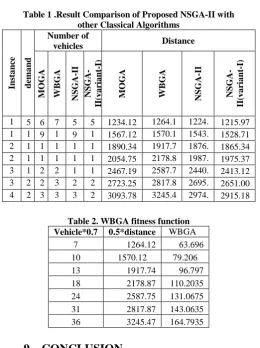
All the programs are implemented in mat lab. The program was run on an Intel Pentium IV 1.6 MHz PC with 512 MB memory. In this paper we discussed different types of evolutionary algorithm. We discussed MOGA, WBGA, NSGA-II and proposed NSGA-II (variant-I). We implemented all the algorithms by solving VRP. In table 1 we narrated experimental results of all the algorithms by taking different population size. Column 3, 4, 5 and 6 explains number of vehicles required to visit customers by using MOGA, WBGA, II and NSGA-II (variant-I) algorithms. Column 7, 8, 9 and 10 explains total distance required to visit customers by using MOGA, WBGA, NSGA-II and NSGA-II (variant-I) algorithms. Table 2 narrates computational result of WBGA by applying explained fitness function in section 7.2. By comparing our proposed algorithm with classical algorithms, NSGA-II (variant-I) gives better results. Figure 5 and 6 shows result comparison of MOGA, WBGA, NSGA-II and NSGA-II (variant-I) for vehicles and total number of distance.

Table 1 .Result Comparison of Proposed NSGA-II with other Classical Algorithms

Insta n ce d em a n d Number of

vehicles Distance

MOG A WBG A NSGA -II NSGA -II (v a ria n t-I) MOG A WBG A NSGA -II NSGA -II (v a ria n t-I) 1 0 0

5 6 7 5 5 1234.12 1264.1 2 1224. 32 1215.97 1 5 0 1 0

9 1 0

9 1 0

1567.12 1570.1 2 1543. 19 1528.71 2 0 0 1 2 1 3 1 3 1 2 1 2

1890.34 1917.7 4 1876. 57 1865.34 2 5 0 1 5 1 6 1 8 1 4 1 2

2054.75 2178.8 7 1987. 98 1975.37 3 0 0 1 9 2 1 2 4 1 9 1 7

2467.19 2587.7 5 2440. 99 2413.12 3 1 0 2 3 2 7 3 1 2 4 2 1

2723.25 2817.8 7 2695. 09 2651.00 4 7 0 2 7 3 4 3 6 3 1 2 8

3093.78 3245.4 7

2974. 58

2915.18

Table 2. WBGA fitness function Vehicle*0.7 0.5*distance WBGA

fitenss

7 1264.12 63.696

10 1570.12 79.206

13 1917.74 96.797

18 2178.87 110.2035

24 2587.75 131.0675

31 2817.87 143.0635

36 3245.47 164.7935

9.

CONCLUSION

In this paper we discussed different classical evolutionary algorithms. We proposed an algorithm NSGA-II (variant-I). To generate offspring for next generation, new crossover and mutation methods are introduced i.e. Random position Crossover Method (RPCM) and Random Incremented Mutation Technique (RIMT). We describe implementation of VRP using MOGA, WBGA, NSGA-II and proposed NSGA-II (variant-I).The proposed methods gives better result as compared to classical algorithms.

1 2 3 4 5 6 7

0 5 10 15 20 25 30 35 instance----> ve hi cl e MOGA NSGA-II NSGA-II(Variant-I)

Fig 5: Experimental result comparison of MOGA, NSGA-II, NSGA-II (variant-I) for

10.

REFERENCES

[1] Paredis, J.1998. The handbook of evolutionary computation. Oxford University Press, Chap. Coevolutionary Algorithms.

[2] DeJong, K. and Potter, M. 1995. Evolving Complex Structures via Cooperative Coevolution Evolutionary Programming, MIT Press Journal, pp. 307-317.

[3] Dhaenens, C., Lemesre, J. and Talbi, E. 2009. A new exact method to solve multi-objective combinatorial optimization problems. European Journal of Operational Research, vol. 200, No. 1, pp. 45-53.

[4] D’Souza, R.G.L., Sekaran, K.C. and Kandasamy, A. 2010. Improved NSGA-II Based on a Novel Ranking Scheme. Journal of Computing, vol. 2, No. 2.

[5] Garey, M.R. and Johnson, D.S. 1979. Computers and Intractability, A Guide to The Theory of NP-Completeness. New York: W. H. Freeman and Company,1979.

[6] Chand, P. and Mohanty, J.R. 2011. Multi Objective GeneticApproach for Solving Vehicle Routing Problem with Time Window. In Proceedings of the CCSEIT Conference on Computer Science Engineering and InformationTechnology, IEEE Press, Sep. 2011,vol.204, pp. 336-343.

[7] Ombuki, B., Ross, J., Brian, J. and Hanshar, F.2006. Multi Objective Genetic Algorithms for Vehicle Routing Problems with Time Windows. IEEE Journal of Applied Intelligence, vol.24, pp. 17-30.

[8] Deb, K. 2001. Multi- Objective Optimization Using Evolutionary Algorithm. Chichester, UK: John Wiley & Sons, Ltd.

[9] Goldberg 2007. Genetic Algorithms in Search,Optimization, and Machine Learning , Addison-Wesley.

[10] Chand, P. and Mohanty,J.R. 2013. A Multi-objective Vehicle Routing Problem using Dominant Rank Method. International Journal of Computer Application, pp. 29-34. [11] Lohn, J., Kraus, W. and Haith, G. 2002. Comparing a

Coevolutionary Genetic Algorithm for Multiobjective Optimization. In Proceedings of the IEEE Congress on Evolutionary Computation, pp. 1157-1162.

[12] Dietz, C., Azzaro-Oantel, L., Pibouleau, S. and Domenech, 2008. Strategies for multiobjective genetic algorithm development: Application to optimal batch plant design in process systems engineering. Elsevier Science, Computers & Industrial Engineering, vol. 54, No. 3, pp. 539-569. [13] Cvetkovic, D. and Parmee, I.C. 1999. Genetic

algorithm-based multi-objective optimisation and conceptual engineering design. In Proceedings of the CEC Conference on Evolutionary Computation, vol.1.

[14] Abdou, W., Bloch,C., Charlet, D. and Spies, F. 2012. Multi-Pareto-Ranking evolutionary algorithm. Journal of Evolutionary Computation in Combinatorial Optimization, pp.194-205.

[15] Chaiyaratana, I.N. and Zalzala, A.M.S. 1997. Recent developments in evolutionary and genetic algorithms: theory and applications. In Proceedings of The GALESIA Conference on Genetic Algorithms in Engineering Systems: Innovations and Applications, pp. 270-277.

[16] Stanley, K.O. and Miikkulainen, R. 2006. Evolving Neural Networks through Augmenting Topologies. Journal of Evolutionary Computation, vol. 10, No. 2, pp. 99-127 [17] Venkadesh, S., Hoogenboom, G., Potter, W. and

McClendon, R. 2013. A genetic algorithm to refine input data selection for air temperature prediction using artificial neural networks. Journal of Applied Soft Computing, vol. 13, No.5, pp.2253-2260.

[18] Devert, A. Weise, T. and Tang, K. 2012. A Study on Scalable Representations for Evolutionary Optimization of Ground Structures. Journal of Evolutionary Computation, vol. 20, No.3, pp.453-472.

[19] Chandra, A. and Yao, X. 2006. Ensemble Learning Using Multi-Objective Evolutionary Algorithms. Journal of Mathematical Modelling and Algorithms, vol. 5, No.4, pp.417-445.

[20] Konaka, A., Coitb, D.W. and Smith, A.E. 2006. Multi-objective optimization using genetic algorithms. A tutorial, Reliability Engineering and System Safety, Elsevier Press, vol. 91, pp. 992-1007.

[21] Hajela, P. and lin, C.Y. 1992. Genetic search strategies in multicriterion optimal design, Struct Optimization. Journal of Engineering Optimisation, vol.4, No.2, pp.99–107.

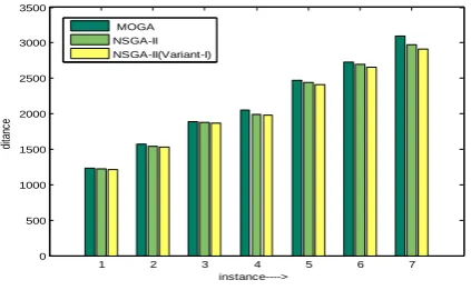
1 2 3 4 5 6 7

0 500 1000 1500 2000 2500 3000 3500

instance---->

di

ta

nc

e

MOGA NSGA-II NSGA-II(Variant-I)

Fig 6: Experimental result comparison of MOGA, NSGA-II, NSGA-II (variant-I) for