Input rich Writing Tasks and Student Writing on an English Language Proficiency Test

Georgia State University

ScholarWorks @ Georgia State University

Economics Dissertations

Department of Economics

Fall 8-24-2017

ESSAYS ON THE ENVIRONMENT AND

DEVELOPMENT

Rhita Pinta Berliana Simorangkir

Georgia State University

Follow this and additional works at:

https://scholarworks.gsu.edu/econ_diss

This Dissertation is brought to you for free and open access by the Department of Economics at ScholarWorks @ Georgia State University. It has been accepted for inclusion in Economics Dissertations by an authorized administrator of ScholarWorks @ Georgia State University. For more information, please [email protected].

Recommended Citation

Simorangkir, Rhita Pinta Berliana, "ESSAYS ON THE ENVIRONMENT AND DEVELOPMENT." Dissertation, Georgia State University, 2017.

ABSTRACT

ESSAYS ON THE ENVIRONMENT AND DEVELOPMENT

By

RHITA PINTA BERLIANA SIMORANGKIR

DECEMBER 2017

Committee Chair: Dr. Paul J. Ferraro

Major Department: Economics

Two essays in this dissertation explore how developing countries effort to improve development

outcomes and to protect their forest areas affect deforestation.

The first chapter investigates the effect of a conditional cash transfers (CCT) program, a rapidly

growing poverty alleviation program in developing countries, on deforestation. Although an increasing

number of studies measure the effects of environmental programs on poverty, little empirical evidence exists

about the effects of poverty programs on the environment. I estimated the effect of substantial and

persistent income transfers to poor households in Indonesia on deforestation. To control for non-random

selection of administrative areas receiving the CCT, I combine semi-parametric matching methods, which

control for observable pre-treatment confounding characteristics, with a difference-in-differences (DID)

design that uses a fixed effect, panel data regression estimator to control for unobservable but

time-invariant confounders. This study combines administrative data from the transfers program and the

Indonesian government, remote sensing data from satellites, and a deep understanding of how the CCT was

scaled up across villages and over time. I found that exposure to the CCT decreases annual forest cover

loss in a village by an estimated 20%, on average. Thus, in Indonesia, efforts to reduce poverty can also

yield environmental co-benefits.

In the second chapter, I examine how a concerted effort to reduce deforestation in a developing

country can be successful. Whether countries with tropical forests can innovate in the policy domain to

substantially reduce deforestation is an open question. I examine this question empirically by analyzing

Brazil’s much-lauded effort to fight deforestation. In 2004, Brazil was ranked the third-largest emitter of

carbon emissions, driven largely by deforestation in the Amazon basin, the worlds largest rainforest and

home to about 10% of the worlds biodiversity. I seek to estimate the effect of a large anti-deforestation

program, the Action Plan for the Prevention and Control of Deforestation (PPCDAm), on deforestation in

high-resolution satellite panel data on global forest cover change. From 2005-2009, the PPCDAm

successfully avoided deforestation of by 88,841 km2. This avoided deforestation is associated with CO2

ESSAYS ON THE ENVIRONMENT AND DEVELOPMENT

BY

RHITA PINTA BERLIANA SIMORANGKIR

A Dissertation Submitted in Partial Fulfillment of the Requirements for the Degree

of

Doctor of Philosophy in the

Andrew Young School of Policy Studies of

Georgia State University

GEORGIA STATE UNIVERSITY

Copyright by

RHITA PINTA BERLIANA SIMORANGKIR

ACCEPTANCE

This dissertation was prepared under the direction of Rhita Pinta Berliana Simorangkir’s Dissertation

Committee. It has been approved and accepted by all members of that committee, and it has been

accepted in partial fulfillment of the requirements for the degree of Doctor of Philosophy in Economics in

the Andrew Young School of Policy Studies of Georgia State University.

Dissertation Chair: Dr. Paul J. Ferraro

Committee: Dr. Jonah Busch

Dr. Jorge Martinez-Vazquez Dr. Carlianne E. Patrick

Electronic Version Approved:

Dr. Sally Wallace, Dean

Andrew Young School of Policy Studies Georgia State University

ACKNOWLEDGEMENTS

This dissertation would not have been possible without the guidance and encouragement of my

advisors Paul J. Ferraro, Jonah Busch, Carlianne E. Patrick, and Jorge Martinez-Vazquez.

A significant development of my professional career in my graduate program was due to guidance from

Paul J. Ferraro. For the first year of my work as his research assistant, I had the privileged to be trained

intensively in exploring research ideas, identifying ideas worth pursuing, thinking critically of my own

work, and conducting research, in particular causal inference research. Although he had left GSU during

my dissertation-writing years, completing this dissertation was possible because of his full commitment and

sharp intuition to understand and challenge my ideas. For all of his guidance and support, I am incredibly

grateful.

During the dissertation process, many mentors, colleagues, and friends have been very generous with

their time to help me with my papers, presentations, and life happiness. In particular, I would like to

thank Paula Stephan for her valuable mentoring and support. I am also thankful to Daniel Kreisman and

Rusty Tchernis for their advice and supports in my job market preparation. I thank Ira, Florian, Sherry,

Alex, Pelin, Anomitro, Dustin, Kalee, Janet, Subha, Ankita, and Valya who made my Ph.D an enjoyable

learning and life experience. I also thank my Buckhead Church Small Group members (Emily, Kaylee,

Leslie, Morgan, Christina, Charry, Antoya, Elizabeth, and Ashley) for encouraging me during tough times

and celebrating life with me during all times.

For their unconditional love and support, I thank my mom, Isnaeni Simorangkir, and my family, Mbak

Ria, Mbak Rhina, Kenneth, Jemma, Ibby, Ka Didit, and Ka Gistang. I also would like to thank Mona,

Jim, Cora, Sam, Logan, Ally, Keeper and Fiona for giving me a place I can call (U.S.) home in Boulder.

I dedicate this dissertation to my dad. Although you are no longer here with me, you have always

TABLE OF CONTENTS

Acknowledgements iv

List of Figures vii

List of Tables viii

Chapter 1. Environmental Consequences of Poverty Alleviation Programs: Evidence from

Conditional Cash Transfers in Indonesia 1

1.1 Introduction . . . 1

1.2 The Program Keluarga Harapan (PKH) . . . 3

1.2.1 Mechanisms . . . 4

1.2.2 Selection of PKH . . . 6

1.3 Identification Strategy & Data . . . 7

1.3.1 Identifying Assumptions . . . 8

1.3.2 Pre-processing using Matching and Fixed Effect Panel Design . . . 10

1.3.3 Data . . . 12

1.4 Results . . . 14

1.4.1 Balance Test and Summary Statistics . . . 14

1.4.2 FE Results . . . 19

1.4.3 Robustness Checks . . . 20

1.4.4 Heterogeneity . . . 22

1.5 Discussion and Conclusion . . . 24

Chapter 2. A Synthetic Control Design to Estimate the Impact of Brazil’s Action Plan for the Prevention and Control of Deforestation in the Legal Amazon (PPCDAm) 25 2.1 Introduction . . . 25

2.2 Plan for the Prevention and Control of Deforestation in the Legal Amazon (PPCDAm) . . . 28

2.3 Identification Strategy & Data . . . 29

2.3.1 Identification Strategy . . . 29

2.3.2 Data . . . 31

2.4 Pool of Countries . . . 34

2.5 Results . . . 36

2.5.2 SCM . . . 38

2.6 Sensitivity Analysis . . . 43

Conclusion 48

Appendices 49

References 51

List of Figures

1.1 Directed Acyclic Graph of CCT’s Effect on Deforestation . . . 5

1.2 The PKH Assignment . . . 6

1.3 High-resolution Satelite Mapping (Hansen, 2013) . . . 13

1.4 Village Boundaries (Statistics Indonesia, 2013) . . . 13

1.5 Density Function of Number of PKH Eligible HHs . . . 16

1.6 Pre-Treatment Forest Loss (2001-2008) . . . 17

1.7 Density Function of Propensity Scores Before Matching . . . 18

1.8 Removing Immediate Neighbors . . . 21

2.1 Ratio of Deforestation to Forest Cover . . . 27

2.2 Annual Forest Cover Loss from Hansen and PRODES Datasets . . . 32

2.3 Trimming Outliers . . . 35

2.4 Annual Forest Cover Loss 2001-2012 . . . 37

2.5 Synthetic BLA . . . 39

2.6 The effect of the PPCDAm in the BLA . . . 41

2.7 Placebo Test of the PPCDAm . . . 43

2.8 The effect of the PPCDAm in the BLA (Removing Cambodia) . . . 45

2.9 Placebo Test of the PPCDAm (Removing Cambodia) . . . 45

2.10 Synthetic BLA: Adding All Covariates . . . 46

2.11 Gaps and Placebo Tests from PRODES data . . . 47

List of Tables

1.1 Data and Sources . . . 15

1.2 Covariates Balance with Unmatched and Matched Samples . . . 15

1.3 Fixed Effect Regression Results . . . 19

1.4 Forest Types . . . 20

1.5 Robustness Checks . . . 21

1.6 Sensitivity Analysis (Rmax= 1.3R2) . . . 22

1.7 Fixed Effect Regression Results: Heterogeneity in Baseline Poverty . . . 23

1.8 Fixed Effect Regression Results: Heterogeneity in Geographical Characteristics . . . 23

2.1 56 Tropical Rainforest Countries Donor Pool . . . 34

2.2 Summary Statistics . . . 36

2.3 Covariates: 57 Tropical Rainforest Countries . . . 39

2.4 Country Weights . . . 40

2.5 Avoided Deforestation and CO2 Storage . . . 42

2.6 Covariates: 56 Tropical Rainforest Countries (Removing Cambodia) . . . 44

A1 Common Support Assumptions . . . 49

Chapter 1. Environmental Consequences of Poverty Alleviation

Programs: Evidence from Conditional Cash Transfers in Indonesia

1.1

Introduction

Given that most carbon and biodiversity-rich tropical rainforests are located in developing countries, it is

not surprising that this biome highly correlates with socio-economic poverty indicators (Fisher and

Christopher, 2007). Thus, policy makers from these countries face the competing uses of these forests: as a

repository of biodiversity and ecosystem services or as an income-generating sector (agriculture, mining,

etc.). Historically, these countries have been less focused on protecting the environment and more focused

on achieving development objectives, such as poverty reduction (Bojo and Reddy,2002;Adams et al.,

2004).

To achieve their economic development objectives, governments are increasingly implementing

conditional cash transfers programs (CCTs). CCTs transfer cash or other resources to poor households.

These transfers are conditional on household members accomplishing specific tasks that are believed to

promote development (e.g., school attendance, pre- and post natal health care visits). Over half of the

thirty tropical countries with the most forest cover now have CCTs program, and others are planning to

create them.

Despite the widespread growth of CCTs program in ecologically-rich countries, previous research

focused on evaluating the effects of CCTs on their targeted outcomes: income, education, and health

indicators (Handa and Davis,2006;Fiszbein and Schady,2009;Barham,2011;Glewwe and Kassouf,2012;

Barham and Rowberry,2013). Only one study has examined the impact of CCTs program on

environmental outcomes (Alix-Garcia et al.,2013). However, given the regression discontinuity

methodology employed by these authors, their results may not generalize to a larger affected population.

In this paper, I revisit the effect of CCTs program on deforestation and focus on a large proportion of

the affected population in the world’s top deforester country, Indonesia. The extent to which CCTs will

affect environmental outcomes in tropical countries is unknown. The poverty-deforestation hypothesis

literature has tried to identify the conditions under which changes in poverty affect deforestation rates, but

conclusions vary. For example, in the context of a theoretical model of a small-scale agricultural

producer,Angelsen(1999) concludes that when labor markets are imperfect (as they are in tropical

countries), deforestation decreases as agriculture productivity or output prices increase. Using a different

between an exogenous change in income and land clearing is ambiguous.

Given the ambiguous predictions from theory, empirical tests of the relationship between deforestation

and income-transfer programs are critical. An earlier literature attempts to estimate the relationship

between income and deforestation across countries using panel designs with random effect and fixed-effect

estimators (Cropper and Griffiths,1994;Koop and Tole, 1999). Given concerns about country-specific

unobserved characteristics that might bias the estimators in these designs, more recent studies use

within-country analysis rather than cross-country analysis (Alix-Garcia et al.,2013;Foster and

Rosenzweig,2003;Khan and Khan,2009;Purnamasari,2010;Zwane,2007). With two exceptions

(Alix-Garcia et al.,2013; Foster and Rosenzweig,2003), most of these studies do not make strong efforts to

eliminate unobserved confounding factors that affect both income and deforestation (violating exclusion

restriction for the instrumental variable approach). Without such efforts, the estimators might suffer from

endogeneity bias.

The two exceptions report conflicting conclusions about the effect of income growth on deforestation.

The results inFoster and Rosenzweig(2003) imply that overall income growth (not income growth from a

specific anti-poverty program) reduced deforestation in India through its positive impact on demand for

forest products. In contrast, the results ofAlix-Garcia et al.(2013) imply that the poverty reduction from

a Mexican CCT (Oportunidades) led to an increase in deforestation. The results from the two studies may

differ because their contexts are different: Foster & Rosenzweig focus on India and do not attempt to

explain the source of income growth, whereas Alix-Garcia et al. focus on Mexico and focus on income

growth that comes from an anti-poverty program. The results may also differ because the study designs

differ: Foster & Rosenzweig use an instrumental variable design and Alix-Garcia et al. use a regression

discontinuity design. Thus each estimates a subgroup-specific local treatment effect, which may not reflect

impacts experienced in the larger population.

In light of these contradictory studies and the need for empirical studies that focus on specific

anti-poverty programs using designs capable of estimating broad program effects, I test the effect of village

level exposure to Indonesia’s CCTs program on deforestation. My analysis is motivated by the evidence

from the pilot implementation of Indonesia’s CCTs program that shows an income increase for the

beneficiary households but no effects on education or long-term health outcomes (Alatas,2011). Since

CCTs program can conceivably affect deforestation through its income or conditionalities, the

aforementioned evidence highlights the potential mechanism through which CCTs could affect

deforestation. Through increase in income, CCTs program can have two countervailing effects on

deforestation. For some beneficiary households, additional income from the program can increase the

others, the income will ease households’ liquidity constraints and make extensive agriculture feasible, hence

increasing deforestation.

Prior research has not been able to clearly identify the causal effect of income on deforestation due to

endogeneity issues. In particular, unobserved confounding factors affect both increase in income and

deforestation. Based on the plausibly exogenous variation of increase in income from the assignment of

Indonesias CCTs program, I can estimate the effect of income on deforestation. Using this spatial variation

information in program exposure at the village level, I employed econometric methods to control for

time-varying, observable sources of bias and time-invariant unobservable sources of bias. Specifically, I

combined semi-parametric matching on observable pre-treatment confounding characteristics, followed by

panel data estimators that seek to control for unobservable, but time-invariant village-level confounders.

This study estimates a program impact that is policy-relevant for Indonesia, i.e., the average

treatment effect on the treated, which is the average impact on village-level deforestation of PKH exposure

on participating villages. Using geo-referenced, administrative data from the PKH program as well as

panel satellite data on changes in forest cover, I regressed villages’ forest cover loss on both time-varying,

observable sources of bias and time-invariant unobservable sources of bias. I found that, on average, village

exposure to the PKH decreased forest cover loss by 3.5 hectares compared to the matched untreated group

(p= 0.041).

Compared to untreated villages, villages exposed to the program have lower forest cover loss: 20% loss

annually. These results are consistent after performing robustness checks over estimation specifications.

The effect size of the PKH-treatment effect is 0.03 which is about half of the minimum effect size of studies

reported in recent reviews of payments for ecosystem services (PES) programs, which are designed

specifically to protect forests.

This paper is organized as follows. Section II describes the key features of the Program Keluarga

Harapan and its potential effect on deforestation. Section III describes the identification strategy and the

data sources. I report summary statistics, test for balance across treated and untreated groups, and

present main results in Section IV. I conclude in section V.

1.2

The Program Keluarga Harapan (PKH)

In this section, I briefly summarize the key features of the PKH; seeSparrow(2008);Alatas(2011);

BAPPENAS(2008) for a more comprehensive description. The Government of Indonesia (GOI) first

implemented a targeted household CCTs program, theProgram Keluarga Harapan (PKH), in 2007 as a

in seven provinces in Indonesia, none of which had dense forest cover. From 2008 onward, the PKH

coverage area was expanded to other provinces, including those with dense forest cover. In this study, I used

the scale up program because it includes areas with dense forest cover. In contrast to the pilot program,

the selection of the PKH sub-districts was no longer random. According to the PKH documentation

(Sparrow,2008;Alatas,2011), the GOI used observable criteria to assign the PKH at the sub-district level.

The PKH transfers cash to mothers in poor households on a quarterly basis. The amount of annual

transfer varies between 600,000 to 2,200,000 rupiahs, which translates to 45 to 165 USD, based on

household eligibility conditions. These amounts are equivalent to 15 to 20 percent of the estimated

consumption of poor households. To be eligible to receive the PKH transfers, a household must be

categorized as ”extremely poor” and must have either one or more of the following conditions: i) pregnant

or lactating mothers, ii) child aged less than 6 years, iii) children of primary school age, iv) children of

secondary school age.

By attaching the cash transfers to health and education obligations, the PKH aims to improve

extremely poor households’ human capital and break the intergenerational transmission of poverty. The

health obligations include pre-natal check-ups, iron tablet consumption, and birth assistance by a trained

professional for pregnant mothers. Lactating mothers have to compete post-natal care visits. Households

with children aged 0-6 years must complete childhood immunizations, take vitamin A and fulfill

growth-monitoring check-ups. To meet the education obligations, households with children aged 6-15 years

must enroll their children at either primary school or junior secondary school and the children must attend

a minimum of 85% of the school days. Finally, households with children aged 16-18 years who have not

completed nine years of primary and secondary school must enroll their children in an education program

to complete the requisite amount of education.

1.2.1 Mechanisms

The PKH can affect deforestation both through the cash transfers and the conditionalities attached to the

PKH. Figure 1.1 summarizes the mechanisms through which CCT could affect deforestation.

Cash transfers from the program relax households’ budget constraints. For agricultural households

with non-separable production and consumption functions and liquidity constraints, exogenous income

transfers would likely change household decisions in both production and consumption sectors (Singh et al.,

1986). In rural areas in developing countries, liquidity and credit constraints limit spending on investment,

consumption, and the choice of income generating activities (Rosenzweig and Wolpin,1993;Barrett et al.,

2005). In the case of Indonesia,Bazzi et al.(2015) analyze liquidity constraints for poor households who

CCTs

Transfer cash

Conditionalities & monitoring

Budget constaint

Social reciprocity

Scrutiny

Consumption smoothing Capital & labor Investment

Consumption

School attendance

Health

Scrutiny

Household’s labor supply

Household’s labor supply & productivity

Deforestation

Fixed sub-district and villages characteristics

Weather

Figure 1.1: Directed Acyclic Graph of CCT’s Effect on Deforestation

cash transfers affect poor households’ consumption decisions and their consumption-smoothing pattern in

the absence of credit access.

Furthermore, the absence of an agricultural insurance market in these areas limits households’ ability

to smooth their consumption. Due to income volatility in the agricultural sector, poor households with

limited credit access diversify their activities to smooth income fluctuations (Dercon,2002); for example

they may use forest products to generate additional income. Several studies show empirical analyses on the

use of forest products as a coping mechanism to mitigate income shocks for low-income households in the

Brazilian Amazon (Pattanayak and Sills,2001), in Peru (Takasaki et al.,2004), and in Malawi (Fisher and

Shively,2005). Regular cash transfers from the PKH could potentially alter their consumption smoothing

strategy by discouraging forest products use, therefore decreasing deforestation.

Conditional cash transfers might also affect citizens’ reciprocity. In one example, conditional cash

transfers program affect how people reciprocate to the elected party providing the program (Galiani et al.,

2016). Observing that villagers in Indonesia have high awareness of negative environmental impacts of

deforestation (Meijaard et al.,2013), they migh reciprocate the government’s cash transfers program by

deforestation through changes in household labor supply and perceived scrutiny.

1.2.2 Selection of PKH

To identify the causal effects of the PKH on deforestation, this study exploits the way in which the PKH

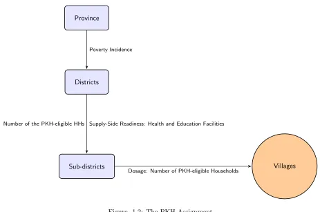
was scaled up over time and space (see Figure 1.2).

Province

Districts

Sub-districts Villages

Poverty Incidence

Supply-Side Readiness: Health and Education Facilities Number of the PKH-eligible HHs

Dosage: Number of PKH-eligible Households

Figure 1.2: The PKH Assignment

To understand how the PKH was implemented, I read through written documentation on the PKH

assignment. Then, to verify and deepen my understanding of the PKH assignment, I conducted a field

survey in August 2016. The survey comprised interviews with the PKH program administrators in Jakarta,

and surveys of head of villages in forested areas in Bali, Sumatera, and Kalimantan.

Written documents from the early implementation of the PKH describe the central government first

assigning PKH eligibility to a province, which is the largest administrative unit, based on several province

attributes: poverty rate, proportion urban, proximity to the coast or islands, and access (Sparrow,2008).

Within a province, eligible districts were selected based on development considerations including a high

incidence of poverty and a high incidence of poor health and education outcomes, and approval from the

district government. Eligible sub-districts were selected based on the number of PKH-eligible households

referred to a sub-district’s ability to accomodate the potential increased demand for health and education

services. To determine a sub-district’s supply-side readiness, the GOI assessed existing health and

education facilities and providers.

To confirm the assignment criteria described in the written documents, I asked the PKH program

administrators (UPPKH) at the Social Ministry of Republic of Indonesia to describe the criteria used for

assigning the PKH to a sub-district. Their responses match the written documents, with some additional

details. In the scaling up phase of the PKH, the number of the PKH eligible households played an

important role in determining the assignment of the PKH to a sub-district. Among the supply-side ready

sub-districts, sub-districts with a high number of the PKH eligible households were prioritized to receive

the PKH earlier than others. This prioritization arose from pressure to expand the PKH to cover all of the

provinces in Indonesia and the PKH’s budget constraint. The PKH administrator at a sub-district level of

administration, which is a unit that is independent of general administrative government, gives the PKH

directly to eligible PKH households. This targeting procedure implies that not all of villages in the PKH

assigned sub-district received the PKH. Only villages with eligible PKH households received the PKH.

Figure 1.2 shows how the central government assigned the PKH from a province to a village level.

One of the concern on applying these observable criteria is that villages might manipulate their

poverty level in order to receive the PKH assignment. This manipulation might confound the PKH

assignment and deforestation. Fortunately, the PKH was assigned on a top-down approach, meaning that

the PKH’s program administrator at the central government assign the PKH to a lower level of

administrator. Furthermore, the list of eligible households was drawn from survey conducted in 2005, two

years prior to the PKH implementation. Hence, it is unlikely that village officials can influence the PKH

assignment in their own village.

1.3

Identification Strategy & Data

Using a potential outcome framework, I identified the causal effect of the PKH on forest cover loss in

Indonesia by estimating the Average Treatment Effect on the Treated (ATT). The ATT represents the

effect of the PKH on forest cover change in those villages that were exposed to the PKH.

Formally, forest cover loss is denoted as Y, while the PKH is denoted as D. Treatment takes on two

values: D=1 indicates PKH assignment while D=0 indicates PKH non-assignment. The Average

AT T =E[Y1−Y0|D= 1] (1)

where [Y1|D= 1] = the observed outcome of the treated unit in the presence of the intervention and

[Y0|D= 1] = the counterfactual outcome of the treated unit in the absence of the intervention.

Since one can never observe the counterfactual outcome of the treated unit in the absence of

intervention, randomized allocation of the treatment to some units ensures that the expected outcome of

the untreated group is equal to the expected counterfactual outcome for the treated group. In other words,

if the assignment of the PKH to villages were random, a simple estimator of the difference in mean

outcomes between PKH and non-PKH villages is an unbiased estimator of the ATT.

In the forested areas of Indonesia, however, the assignment of the PKH was not random. With

non-random assignment, the expected changes in forest cover loss in PKH and non-PKH villages are likely

to be different in the absence of the PKH. To obtain appropriate counterfactuals for the treated villages,

this paper controls for different baseline characteristics that affect both the PKH assignment and changes

in forest cover loss. These characteristics are chosen based on the PKH selection criteria for villages and

historical forest cover loss. The associated estimand becomes:

AT T =E[Y1−Y0|X, D= 1] (2)

The treated group consists of villages that received the PKH from 2008 to 2012. I constructed a

counterfactual group for the PKH treated villages from villages that did not receive the PKH by the end of

2012 within the same provinces. Equation (2) means that once I conditioned on X, the treatment

assignment is ”as if” randomly assigned. According toHeckman et al.(1998), the lowest bias values arise

when X includes a set of variables that affect both program participation and the outcome. Thus, the

conditioning set X comprises observable PKH-assignment indicators and forest change outcomes, including

pre-treatment forest losses and forest cover. Pre-treatment outcomes are included in the observed

conditioning set to block a variety of back-door paths via unobservable variables that affect forest cover in

both the past and the future.

1.3.1 Identifying Assumptions

In order to make a causal inference, this study assumes that the potential outcomes for any unit do not

formally known as the Stable Unit Treatment Value Assumption (SUTVA). Based onRubin(1980),

SUTVA is satisfied when there is no interference between units leading to different outcomes depending on

the treatments other units received and there are no versions of treatments leading to technical errors.

SUTVA and other assumptions discussed later are not directly informed by observationsImbens and Rubin

(2015). However, in this study,one might worry that the PKH transfers might generate general equilibrium

effect in which transfers received by a household might affect other households that did not receive the

PKH. This study makes SUTVA more credible by defining the unit to be the village within which eligible

PKH households interact.

Furthermore, to consistently estimate the ATT,Heckman et al.(1997) suggest several assumptions

that need to be maintained: (i) Conditional Independence Assumption; (ii) Common Support Assumption.

To identify the ATT parameter, we need the assumption of conditional independence ofY0 given X; i.e.,

(Y0) |=D|X. Estimate ofY0for units with D=1 would be inferred from data on units with D=0. Given

the conditional independence assumption is true,Heckman et al. (1997) show that the outcomes of

untreated units will have the same distributions with treated units if they were not participated in the

program, after conditioning on X. Thus, if the mean exists:

E[Y0|X, D= 1] =E[Y0|X, D= 0] =E[Y0|X] (3)

Equation (3) means that the expected outcome of the untreated group, the group that did not receive

the treatment, is a valid counterfactual of expected outcome for the treated group.

The common support assumption means that the probability of participating and not participating is

bounded away from zero and one. This assumption rules out the perfect predictability of the treatment

assignment, D, after conditioning for X. To estimate ATT, we only need the possibility of a non-participant

for each participant (Smith and Todd,2005). Thus, the common support is:

P(D= 1|X)<1 (4)

In this paper, I used a sensitivity analysis that assumes that the selection on observables provides

information on the selection on unobservables. This method was originally developed by (Altonji et al.,

2005) and later on extended byOster(2016). In addition to observing coefficient movements, Oster

formally incorporated the R-squared movements in the bias adjustment calculation to evaluate the

robustness of the specification from omitted variable bias. By setting the maximum R-squared to 1.3 of the

selection on unobservables relative to observables, , that would be necessary to have a zero treatment

effect. Altonji et al. suggest a threshold point of equals to one. This threshold suggests that the

observables are at least as important as the unobservables. Finally, I assume that if there exist any

unobservable confounders, they are time-invariant.

1.3.2 Pre-processing using Matching and Fixed Effect Panel Design

To address the concern about bias from non-random treatment assignment, I pre-processed the data using

a matching algorithm that strives to make the treated and untreated villages similar on key observable

characteristics known to affect both assignment to the PKH and forest cover change (Ho et al.,2007).

Pre-processing using matching adjusts the data for potential confounding factors semi-parametrically. The

adjustment of the data requires the inclusion of observable characteristics, X, that affect the selection of

area into the PKH recipients and forest cover change in the matching process.

The propensity score estimate is consistent only if matching on the associated propensity score

asymptotically balances the observed covariates (Ho et al., 2007). To achieve covariates balance,

Rosenbaum and Rubin(1983) recommend iteratively checking if matching on the estimated propensity

score produces balance by revising the specification of the propensity score until covariate imbalance is

minimized. Since matching does not use outcome data in the post-treatment period, the practice of

iteratively checking and revising the specification to minimized covariate imbalance is permissible (Rubin,

2008).

Genetic Matching (Diamond and Sekhon,2012) is a matching algorithm that eliminates the need to

manually and iteratively checks the propensity score. It is a generalization of propensity score and

Mahalanobis distance (MD) matching algorithm. Genetic Matching automates the iterative process of

checking and improving overall covariate balance and guarantees asymptotic convergence to the optimal

matched sample. It may or may not decrease the bias in the conditional estimates.

In contrast with experimental studies, the existence of a set of observed conditioning variables that

satisfy both conditional independence and common support assumptions is not guaranteed in observational

studies. Balance in conditioning set X between treated and untreated groups is traditionally used as an

indirect test for the conditional mean independence assumption. I assess balance using graphs and

normalized differences between treated and untreated groups.

In most observational studies, untreated matches for a fraction of treated units cannot be found, thus,

violating equation (4). In this case, there are regions where the support of X does not overlap for D=1 and

D=0 groups. When there is a minimal overlap in the distribution of propensity score between treated an

(Dehejia and Wahba,2002). Several ways are suggested to impose the region of common support. Smith

and Todd(2005) suggest trimming to determine the support region. One drawback of this method is the

estimated treatment effect will no longer be generalized to the entire region. Alternatively, I can impose a

common support condition by using a caliper matching (Cochran and Rubin,1973).

To test how sensitive the analysis to a hidden bias, I relax the unconfoundedness assumption. From

this unconfoundedness, I obtained a range of plausible values for the estimand with the width of these

ranges corresponding to the extent to which I allow the unconfoundedness assumption to be violated.

Matching is unlikely to remove all of the bias in the estimator, both because of imperfect matching in

finite samples and because of unobservable confounding factors. Following the suggestion ofHo et al.

(2007), I impose parametric procedures on the pre-processed data set. Specifically, this study uses a fixed

effect panel design to mitigate the confounding effects of unobservable, time-invariant characteristics.

Suppose there exists forest cover loss spillover among sub-districts; fixed effect panel regression design helps

remove the constant spillover. As fixed effect panel regression design assumes homogenous treatment

effects, the treated and untreated units respond similarly, on average, to common shocks. To the extent

that treatment effect heterogeneity and responses to common shocks are a function of observable

characteristics and time-invariant unobservable characteristics, the combined designs of pre-processing

using matching and fixed effect panel regression will make these assumptions more plausible (Ferraro and

Miranda,2017).

To estimate the effect of a poverty alleviation program on forest cover, this paper uses the

difference-in-differences (DID) method using fixed effect panel regression design. Using treated and

matched untreated units, ATT is estimated by the difference on forest cover outcome between these two

groups.

Yit=β0+β1P KHit+β2Xit+αi+γt+it (5)

The unit of analysis in this paper is the village level of administration. Yitis the forest cover loss in

village i at year t from panel data, 2001 to 2012. The coefficient of interest isβ1, which indicates the effect

of exposure to the PKH program onYit. To help improve the precision of the estimator,Xitcomprises two

time-varying characteristics that are known to affect agriculture and thus forest cover loss: average

temperature and precipitation rate. The fixed effect,αi, captures a villages unobserved time-invariant

characteristics that can affect exposure to the PKH and forest cover loss. The time variable,γt, represents

national-level time-varying characteristics that affect forest cover loss. The random error term is

The unit of analysis is the village, but the PKH was assigned to a sub-district, which comprises

several villages. To control for intra-sub-district correlation, I estimate standard errors clustered at the

sub-district level.

1.3.3 Data

Outcome. I use forest cover loss fromHansen et al.(2013) as a measure of deforestation within a village.

Forest cover loss is defined as the complete removal of tree cover (a stand-replacement disturbance). Tree

cover is indicated by a Landsat pixel covered by all vegetation higher than 5 meters in the beginning of a

year (January) at or above a 75% threshold of canopy cover. Hansen’s dataset was obtained from a

high-resolution satellite, Landsat 7, at a spatial resolution of 30*30 meters to measure forest cover change

from 2000 to 2012 globally. This dataset provides a uniform and consistent measure of forest cover and

forest loss for all global land at a small spatial resolution.

To obtain a dataset on forest cover change for each village in Indonesia, I overlaid the Hansen data set

with Indonesias 2013 village boundaries (Statistics Indonesia) using the gfcanalysis package in R (Zvoleff,

2015). Combining these two datasets minimizes forest cover interpolation around the village’s boundaries.

Since the spatial resolution of the Hansen dataset is sufficiently small, I can measure in details the

variation of forest cover across villages. This study overlaps Hansens data with the Indonesia’s 2013 village

boundary using gfcanalysis package in R (Zvoleff,2015). The spatial mapping of the treated villages was

created using geographical information software ArcGIS 10.3. The resulting data set consists of a panel of

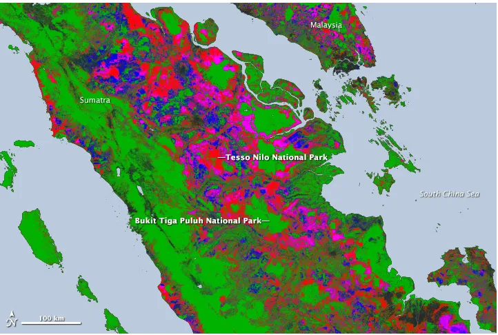
treated and untreated villages forest cover loss from 2001 to 2012. Figure 1.3 and 1.4 show the overlapping

of these two datasets.

Treated Villages. In this paper, treated village is defined as a village that received the PKH between

2008 and 2012 and had a positive forest cover in 2001. Untreated villages are the villages with positive

forest cover in 2001 that did not receive the PKH by 2012. The list of villages that received the PKH from

2008 to 2012 was obtained from the State Ministry of National Development Planning (BAPPENAS). This

treated village dataset gives a village identification using the name and the official 2014 village code from

Statistic Indonesia. After the implementation of a regional autonomy law in Indonesia in 2000

(Brodjonegoro and Martinez-Vazquez,2004), Indonesia experienced a proliferation of administrative areas.

The proliferation ranged from the establishment of new villages to the creation of new districts. Given this

proliferation, the village names or codes could change over time. For this reason, I collapsed the treated

villages to village names and codes in 2007. I chose this year because the targeting of the PKH was based

Figure 1.3: High-resolution Satelite Mapping (Hansen, 2013)

All villages in the sample areas received the PKH starting from 2008, except the villages in one district

in West Sumatera. This particular district in West Sumatera has been removed from the sample because it

received the PKH in the pilot program. Hence, the treatment period of the overall sample starts in 2008.

Administrative Selection Variables. The administrative selection variables consist of three observable

characteristics obtained from TNP2K. These variables include the number of PKH-eligible characteristics,

access to health facilities, and access to education facilities in sub-district level of administration. These

variables were obtained from The National Team for the Acceleration of Poverty Reduction (TNP2K). This

team is one of the coordination team that implements PKH in Indonesia.

Pre-treatment Outcomes. Pre-treatment forest loss used in this paper goes back to 2 years before the

treatment period. Moreover, this study matches on the forest cover at the beginning of the treatment year.

This covariate serves as a normalization of the extent of the forest cover loss across villages.

Others. Another covariate used for the pre-processing using matching is the length of roads within a

village in 2010. Proximity to road has been an important factor affecting deforestation in many tropical

countries (Ferretti-Galon and Busch,2014). Hence, I included length of road as the matching covariate.

Table 1.1 summarizes data and the sources of the data.

1.4

Results

1.4.1 Balance Test and Summary Statistics

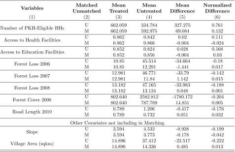
In my analysis, I performed matching within a province and then merged the matched samples for all 16

provinces into a single data set. Table 1.2 reports the covariate balance statistics before and after

matching. As expected given the targeting of the PKH, the treated group has a higher number of

PKH-eligible households and higher access to health and education facilities compared to the untreated

group. The treated group also has, on average, lower pre-treatment forest cover loss and shorter length of

road compared to the untreated group.

After matching, the differences between treated and untreated groups are smaller. Column (5) in

Table 1.2 shows the mean differences in covariates between treated and treated groups while column (7)

shows the normalized differences. Following the suggestion fromImbens and Rubin(2015) (as cited in

Imbens and Wooldridge(2009)), I use the normalized difference threshold of 0.25 to judge the sensitivity of

Table 1.1: Data and Sources

Variable Source

Forest loss & forest cover 2001-2012 Hansen et.al. (2013) version 1.2 Village boundaries 2013 Statistics Indonesia

PKH villages The State Ministry of National Development Planning (BAPPENAS) Number of eligible households in a sub-district the National Team for the Acceleration of Poverty Reduction (TNP2K)

Access to health facilities in a sub-district the National Team for the Acceleration of Poverty Reduction (TNP2K) Access to education facilities in a sub-district the National Team for the Acceleration of Poverty Reduction (TNP2K)

Road length in 2010 Socioeconomic Data and Applications Center (SEDAC) Precipitation rate TRMM 3B43 V.7

Yearly average surface temperature M2TMNXFLX V5.12.4

Slope SRTM 90m Digital Elevation Database v.4.1

Palm oil concessions Indonesia Ministry of Forestry accessed through Global Forest Watch Wood fiber concessions Indonesia Ministry of Forestry accessed through Global Forest Watch Logging concessions Indonesia Ministry of Forestry accessed through Global Forest Watch Protected areas 2010 World Database of Protected Areas

Table 1.2: Covariates Balance with Unmatched and Matched Samples

Variables Matched Mean Mean Mean Normalized

Unmatched Treated Untreated Difference Difference

(1) (2) (3) (4) (5) (6)

Number of PKH-Eligible HHs U 662.059 334.784 327.275 0.761

M 662.059 592.975 69.084 0.132

Access to Health Facilities U 0.862 0.842 0.02 0.111

M 0.862 0.866 -0.004 -0.024

Access to Education Facilities U 0.852 0.824 0.028 0.168

M 0.852 0.856 -0.004 0.03

Forest Loss 2006 U 10.85 45.514 -34.664 -0.18

M 10.85 12.291 -1.441 0.017

Forest Loss 2007 U 12.981 46.771 -33.79 -0.142

M 12.981 11.84 1.142 0.015

Forest Loss 2008 U 13.182 47.165 -33.983 -0.188

M 13.182 13.134 0.048 0.001

Forest Cover 2008 U 802.640 2582.812 -1780.172 -0.204

M 802.640 787.789 14.851 0.005

Road Length 2010 U 0.789 1.206 -0.417 -0.176

M 0.789 0.732 0.051 0.032

Other Covariates not including in Matching

Slope U 3.594 4.532 -0.938 -0.199

M 3.594 3.773 -0.178 -0.042

Village Area (sqkm) U 14.896 37.412 -22.517 -0.222

The most severly imbalanced variable is also the most important for PKH assignment: the number of

PKH-eligible households. After matching, the balance is greatly improved, falling below the 0.25 threshold.

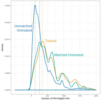
The improvement in covariate balance can be seen directly from the kernel density functions in Figure 1.5.

Compared to the treated group’s density, the density of the untreated group is much farther to the left.

After matching, it overlaps well with the trated group.

0.0000 0.0005 0.0010 0.0015 0.0020 0.0025

0 500 1000 1500 2000

Number of PKH-Eligible HHs

Density

Unmatched

Untreated

Matched Untreated

Treated

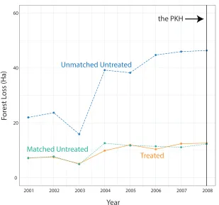
Figure 1.6 shows the common trends in pre-treatment forest cover loss between treated and untreated

villages. The PKH was first assigned in the forested area in Indonesia in 2008. Prior to 2008, the annual

means of forest cover loss for the treated group, the orange solid line, is much lower than for the

unmatched untreated group, the blue dashed line. It also follows a different trend, which makes the

identifying assumptions of the fixed effects, panel data estimator less plausible: if pre-treatment trends of

treated and control units were not, on average, similar prior to treatment assignment, it is harder to belive

that, in the post-treatment period, the untreated group’s trend represents the counterfactual trend of the

treated group in the absence of treatment (conditional on weather variables). In contrast, the level and

trend of forest loss for the untreated group, the teal dotted line, closely follows those of the treated group.

2001 2002 2003 2004 2005 2006 2007 2008 0

20 40 60

Matched Untreated

Treated

Unmatched Untreated

the PKH

Year

For

est L

oss (Ha)

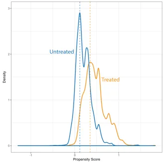
Common Support. To ascertain the plausibility of the common support assumption, I observe the

graphical representation of the propensity scores densities of both treated and untreated groups. Caliendo

and Kopeinig(2005) point out that graphical analysis is sufficient to see the common support. Looking at

Figure 1.7, it is clear that the treated and untreated groups share overlapping regions. Furthermore, I

performed multiple common support tests, including trimming outliers of the common support in terms of

propensity scores (Caliendo and Kopeinig,2005), imposing common support while performing genetic

matching within a province. similar approach proposed byDehejia and Wahba(2002), and inmpsing

caliper matching (Cochran and Rubin,1973). The results in Appendix (Table A1) from all of these tests

suggest reduction in forest cover loss in PKH-treated villages compared to untreated villages.

0 1 2 3

-1 0 1

Propensity Score

Density

Untreated

Treated

1.4.2 FE Results

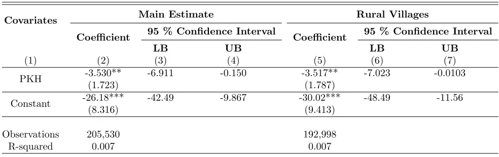
Table 1.3 presents the estimates of PKH treatment effects on village level forest loss. After matching,

column (2-4), Village exposure to the PKH decreases forest loss by an estimated 3.53 hectares (p=0.04).

Removing villages that are located in districts that are categorized as cities by the GOI column(5-7), the

estimated impact declines to 3.5 ha (p=0.049).

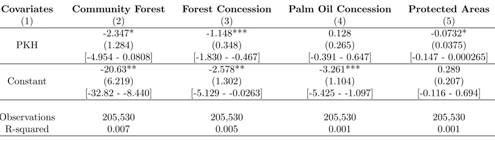
Table 1.4 presents estimated treatment effects by forest type. Community forest, refers to village

forests outside of concession and protected areas. Forest concessions consist of logging and wood fiber

concessions. Estimated reductions in forest loss are largest in the community forests (2.3 Ha, p=0.058),

followed by forest concessions (1.15 Ha, p=0.001), and protected areas (0.07 Ha, p=0.051). The estimated

effect of the PKH in palm oil concessions is positive (0.13 Ha, p=0.630) although it is very imprecisely

estimated and thus much less informative that the other estimates.

Table 1.3: Fixed Effect Regression Results

Covariates Main Estimate Rural Villages

Coefficient 95 % Confidence Interval Coefficient 95 % Confidence Interval

LB UB LB UB

(1) (2) (3) (4) (5) (6) (7)

PKH -3.530** -6.911 -0.150 -3.517** -7.023 -0.0103

(1.723) (1.787)

Constant -26.18*** -42.49 -9.867 -30.02*** -48.49 -11.56

(8.316) (9.413)

Observations 205,530 192,998

R-squared 0.007 0.007

***p <0.01, **p <0.05, *p <0.1 Clustered s.e. at sub-district level

Standard errors in parentheses, 95 % confidence interval in brackets

Table 1.4: Forest Types

Covariates Community Forest Forest Concession Palm Oil Concession Protected Areas

(1) (2) (3) (4) (5)

PKH

-2.347* -1.148*** 0.128 -0.0732*

(1.284) (0.348) (0.265) (0.0375)

[-4.954 - 0.0808] [-1.830 - -0.467] [-0.391 - 0.647] [-0.147 - 0.000265]

Constant

-20.63** -2.578** -3.261*** 0.289

(6.219) (1.302) (1.104) (0.207)

[-32.82 - -8.440] [-5.129 - -0.0263] [-5.425 - -1.097] [-0.116 - 0.694]

Observations 205,530 205,530 205,530 205,530

R-squared 0.007 0.005 0.001 0.001

***p <0.01, **p <0.05, *p <0.1 Clustered s.e. at sub-district level

Standard errors in parentheses, 95 % confidence interval in brackets

Fixed effect controlling for average precipitation, average temperature, and year dummies

1.4.3 Robustness Checks

Eventually Treated Sample. I performed robustness check by estimating the effect of the PKH to those

villages that eventually received the PKH by 2012. I performed this robustness check because those villages

that eventually received the PKH were the best matches for the treated villages. In implementation, I

removed untreated villages that never got treated by the end of 2012. Furthermore, I assumed that the

year in which a village is selected for treatment is ”as if randomly assigned” after conditioning on

community fixed effect and year effects. Table 1.5 shows the result that the PKH reduced forest loss by

almost 5 Ha (p=0.006), a coefficient movement of almost 39%. As an alternative, I also performed random

effect panel regression estimate on this eventually treated sample controlling for administrative selection

covariates (number of eligible PKH households, access to health facilities, and access to education

facilities), geographical characteristics (length of roads, slope, elevation), weather covariates (average

temperature and precipitation), and year effects. I performed estimation on this specification becaue it

allows the inclusion of the selection covariates. The result suggests that the PKH reduces forest cover loss

by 5.1 Ha (p=0.006), a similar estimate to the FE specification. In conclusion, these results emphasize the

deforestation-reducing effect of the PKH.

Removing Neighbors. Theoretically, income increase in the PKH villages can increase demand that

then increases local agricultural prices. Following the method to reduce the bias from spatial spillover by

Andam et al.(2008), I removed untreated villages that shared boundaries with the treated villages and

performed matching with the new set of untreated units. Figure 1.8 shows the graphical representation of

villages, the blue polygons represent untreated villages that shared boundaries with PKH-treated villages,

and the white polygons represent the untreated villages. I removed PKH-untreated neighbors, the blue

polygons. From 16 provinces, I removed 2,142 untreated villages that correspond to 7% from total

untreated villages. In the appendix, I present the covariate balance after removing untreated neighbors.

Similar as the matching specification, normalized differences across covariates are lower than 0.25 after

matching. Column 3 in Table 1.5 shows the results after removing untreated neighbors. The result shows

reduction in forest cover loss and roughly similar estimate with coefficient movement of 26.6%.

Table 1.5: Robustness Checks

Covariates Eventually Treated Sample Removing Neighbors

FE REa _FE

(1) (2) (3) (4)

PKH

-4.935*** -5.134*** -2.590

(1.796) (1.884) (1.771)

[-8.462 - -1.408] [-8.826 - -1.442] [-6.064 - 0.884]

Constant

-19.56*** 1.828 -21.72***

(9.832) (12.22) (8.205)

[-38.87 - -0.250] [-22.11 - 25.77] [-37.82 - -5.625]

Observations 102,765 102,765 205,530

R-squared 0.008 0.008

***p <0.01, **p <0.05, *p <0.1 Clustered s.e. at sub-district level

Standard errors in parentheses, 95 % confidence interval in brackets Controlling for average precipitation, average temperature, and year dummies a_{Additional controls: administrative selection variables and geographical characteristics}

Sensitivity Analysis. One of the concerns from estimating ATT in observational settings is that,

despite all of my efforts to eliminate sources of bias from confounding variables, the design might still suffer

from omitted variable bias. In order to test the sensitivity of the specification to this bias, I measured the

degree of selection on unobservables relative to selection on observables,δdeveloped by (Oster,2016). In

order to perform this sensitivity analysis, I took the matched samples and estimated the OLS from the

cross section data. I regress the PKH assignment and matching covariates on forest cover loss in 2012.

Then, I asked how large aδ has to be in order to change my estimate by performing psacalc command in

stata. I useδ= 1 as the rule of thumb proposed by (Altonji et al.,2005) to measure the degree of selection

on unobservables compared to the selection on observables. Ifδ= 1, the unobservable variable has to be as

strong as the observable covariates in the regression specifications to alter the estimate. Table 1.6 shows

the results for this sensitivity analysis. Column (4) shows the magnitude of delta to change the treatment

effect to zero. Since delta is substantially higher than 1, my specification is not sensitive to hidden bias. In

order to change the estimate to a positive value (Column (5)), delta is also substantialy higher than one.

In conclusion, the primary result is not sensitive to hidden bias.

Table 1.6: Sensitivity Analysis (Rmax= 1.3R2)

Specification Baseline effect (Std. error) [R2_{] R}

max δ˜for β= 0 δ˜forβ =−βˆ

(1) (2) (3) (4) (5)

Main Estimate -5.099*** (1.564)

0.61698 -20.41356 -42.15367

[0.4746]

Rural Villages -5.71*** (1.778)

0.63778 -14.78526 -29.79117

[0.4906]

1.4.4 Heterogeneity

The estimated overal average causal effect of the PKH on deforestation is informative yet of limited value

Imai and Ratkovic(2013). In order to investigate when the treatments do and do not work, I explored the

heterogeneity of treatment effect to test for the existence of lack there of heterogenous treatment effects

and to choose sub-populations for which a treatment is effective or harmful. In terms of the relation

between income from poverty alleviation progam and deforestation, previous work documented a non-linear

relationship between income and deforestationDasgupta et al. (2002). Hence, subpopulations of with high

and low baseline poverty level is one of the subpopulation of interest. Moreover, geographical characteristics

also explored the heterogeneity in sub-populations reside in different geographical characteristics.

In table 1.7, I examined the heterogeneity of the effect of the PKH by baseline poverty level of the

sub-district where PKH villages are located. I divided the sample into low versus high baseline poverty

villages using the median number of PKH-eligible households. I found no systematic differences in the

treatment effects of the PKH on deforestation. In particular, the point estimates of the effect of the PKH

are all negative for both villages with low and high baseline poverty. I also explored heterogeneity of the

PKH effect by the village’s geographical conditions, including slope and village area. Table 1.8 presents the

results for heterogeneity in geographical characteristics. In conclusion, the deforestation-reducing effect of

the PKH exposures to villages appears to be homogenous across the subgroups examined in my analysis.

Table 1.7: Fixed Effect Regression Results: Heterogeneity in Baseline Poverty

Covariates Low Baseline Poverty High Baseline Poverty

Coefficient 95 % Confidence Interval Coefficient 95 % Confidence Interval

LB UB LB UB

(1) (2) (3) (4) (5) (6) (7)

PKH -2.447 -6.337 1.443 -3.415 -7.996 1.167

(1.982) (2.333)

Constant -20.21* -44.06 3.630 -25.80* -50.41 -1.198

(12.15) (12.53)

Observations 99,684 105,846

R-squared 0.009 0.008

***p <0.01, **p <0.05, *p <0.1 Clustered s.e. at sub-district level

Standard errors in parentheses, 95 % confidence interval in brackets

Fixed effect controlling for average precipitation, average temperature, and year dummies

Table 1.8: Fixed Effect Regression Results: Heterogeneity in Geographical Characteristics

Covariates Slope Village Area

Low High Low High

(1) (2) (3) (4) (5)

PKH

-2.726 -3.359* -1.048 -4.832*

(2.478) (1.837) (0.778) (2.808)

[-7.588 - 2.136] [-6.693 - 0.246] [-2.574 - 0.478] [-10.34 - 0.677]

Constant

-32.17** -27.15*** -8.421** -40.31***

(12.70) (9.082) (3.985) (14.18)

[-57.09 - -7.255] [-44.97 - -9.324] [-16.24 - -0.600] [-68.12 - -12.49]

Observations 102,700 102,830 102,700 102,830

R-squared 0.006 0.010 0.008 0.012

***p <0.01, **p <0.05, *p <0.1 Clustered s.e. at sub-district level

Standard errors in parentheses, 95 % confidence interval in brackets

1.5

Discussion and Conclusion

Due to a high spatial overlap between poverty and biodiversity regions (Fisher and Christopher,2007),

understanding the effect of poverty reduction to environmental outcomes becomes crucial. How poverty

alleviation programs might affect environmental outcomes has been difficult to answer due to the

endogeneity between poverty and forest cover. This paper evaluated the environmental consequences of

poverty alleviation program in a developing country. In contrast with prior work evaluating CCTs in

Mexico, this study found that village exposure to the CCT reduced forest loss by 20%. This finding is

robust after adjusting for potential spillover, overlapping regions of common support, and hidden bias.

This opposite conclusion could arise from different contexts (Mexico vs. Indonesia) or from different study

designs. The estimand for this Indonesia study is the average treatment effect on the treated villages. The

estimand for the Mexico study is a local average treatment effect around an eligibility threshold based on a

poverty index, i.e., it measures the treatment effect for only communities just above or just below the

eligibility threshold.

Exploring heterogeneity of treatment effects from baseline poverty levels, slope and village areas, a

village exposure to the PKH reduces forest loss. Finally, compared to the effect sizes from payment for

environmental services (PES), an environmental program that was designed specifically to protect forests,

the effect size from the PKH (0.03) was half of the minimum effect size of studies evaluating PES (0.06).

Future research should attempt to isolate the mechanisms through which a poverty alleviation

program like the PKH can affect deforestation. In a developing country like Indonesia, most of poor people

in rural areas work in agricultural sector. Income in agricultural sector is known to be seasonal and tend to

fluctuate. Poor people who have limited access to credit often use forest products to cope with income

fluctuations from agricultural sector. The regular cash transfers from the PKH might decrease the pressure

on forest.

This paper shows that in the context of Indonesia, effort to reduce poverty is followed by

environmental benefits. The treatment effect estimated in this paper is policy relevant as it uses a large

and heterogeneous sample from all the administrative units that have received the PKH. As Indonesia

currently has no carefully designed environmental policies, the income from the PKH helps reducing the

pressure deforest.

This study contributes to the sparse literature on the environmental impacts of development

programs. It also contributes to a more accurate and informative model of regional deforestation models in

Asia because it uses variation in village-level data. This study also finds that a CCT program can have a

Chapter 2. A Synthetic Control Design to Estimate the Impact of

Brazil’s Action Plan for the Prevention and Control of

Deforestation in the Legal Amazon (PPCDAm)

2.1

Introduction

Emission from deforestation has been a significant contributor of global greenhouse gas emissions (Seymour

and Busch,2016). A traditional policy approach to slow down deforestation has heavily relied on protected

areas and other area based conservation practice. These approaches have successfully reduced deforestation

(Andam et al.,2008;Adams et al., 2004; Ferraro et al., 2013; Jayachandran et al.,2017;Sims and

Alix-Garcia,2016), but the magnitude of the reduction is modest. In the absence of innovations in forest

conservation policy, an area the size of India will be cleared each year in the near future (Busch and

Engelmann,2015). Whether countries with tropical forests can innovate in the policy domain to

substantially reduce these expected losses is an open question.

I examine this question empirically by analyzing Brazil’s much lauded effort to fight deforestation.

Brazil is an ideal setting because it has the world’s largest tropical rainforests - the Amazon- and had

experienced some of the world’s highest deforestation rates for decades. To combat this deforestation in the

Amazon, the Brazilian government implemented, in 2004, the Action Plan for the Prevention and Control

of Deforestation in the Legal Amazon, known by its Portugues acronym as the PPCDAm. Executed

through a colaboration among thirteen ministries, the PPCDAm comprises a set of initiatives for

monitoring, enforcement, and territorial management (Assun¸c˜ao et al.,2015). These initiatives include a

satellite-based monitoring system, additional personnel for field-level monitoring and enforcement

activities, land tenure policy changes, restrictions on agricultural credit to illegal deforesters, and a

blacklist of municipalities that account for 45% of Amazonian deforestation.

This large, anti-deforestation program aimed to reduce, by 2020, deforestation to 20% of its historical

average between 1996 and 2005. During this period, 19,625km2 _{was deforested annually, an area roughly}

the size of the State of New Jersey (average is calculated from data published by the Brazilian

Government; PRODES, INPE). By 2010, the annual deforestation rate had been cut to 7,000km2, a

reduction of more than 60%. Because of this dramatic reduction, the program has been lauded in the

international media and by global organizations as an example of how concerted legal action can

However, the extent to which the dramatic reduction in deforestation can be attributed to the

PPCDAm, rather than other factors affecting deforestation in tropical nations more broadly, has not been

investigated. Most prior studies have attempted to study individual components of the PPCDAm (Arima

et al.,2014;Assun¸c˜ao et al.,2013a,b;Assun¸c˜ao and Rocha,2014;Cisneros et al.,2015). Disentangling the

individual effects of contemporaneously-implemented and spatially-correlated PPCDAm components is

difficult and, moreover, does not address the question of the overall impact of the coordinated initiative.

One study by (Assun¸c˜ao et al.,2015) attempted to simulate the overall impact by estimating a model that

interacted the policy implementation period with a measure of land tightness, which varied within

municipalities inside the Brazilian Legal Amazon and was theorized to moderate the effect of the PPCDAm.

By simulating the overall impact using data from municipalities within the BLA, the design likely

under-estimates the true effect of the PPCDAm because all municipalities are exposed to the initiative.

Estimating the effect of the PPCDAm on deforestation rates is difficult for two reason. First, only one

region the Brazilian Legal Amazon (BLA) has been treated (i.e., exposed to the PPCDAm). With a

treated sample size of one, statistical inference using standard methods is challenging. Second, one can

observe post-PPCDAm Amazonian deforestation rates, but one cannot observe the counterfactual

deforestation trends in the absence of the PPCDAm. Estimating these counterfactual trends requires

finding a suitable comparison region that was not exposed to the PPCDAm or a similar program. Brazil

and its Amazon region, however, are unique. Thus finding a comparison region(s) that represents the

Amazons counterfactual (no PPCDAm) deforestation trend is not straightforward.

Figure 2.1 shows the trend in the annual rate of forest change in the Brazilian Legal Amazon (BLA)

compared with (a) the average rate for 56 wet tropic forest countries and (b) the individual rates of the top

10 tropical countries with the most forest cover. Prior to the PPCDAm in 2004, the trends of the BLA and

the average of the 56 countries are moving in opposite directions. Given that the full pool of tropical

rainforest countries has a similar trend prior to PPCDAm, it would not be credible to assume that the

trends of the full pool could represent the BLAs counterfactual deforestation trend in the absence of the

PPCDAm.

To estimate this counterfactual deforestation trend, and to conduct statistical inference, I combined a

synthetic control design (Abadie and Gardeazabal, 2003; Abadie et al.,2010,2015) and newly available,

high-resolution satellite panel data on global forest cover change from 2001 to 2012 (Hansen et al.,2013).

The data-driven, synthetic control design offers a systematic and transparent method for choosing a

weighted set of comparison region(s) from the donor pool of tropical rainforest nations to serve as a control

group; i.e., I created a synthetic BLA from a weighted mixture of other wet tropical forest countries. The

0.000 0.003 0.006 0.009 0.012 0.015 2012 2011 2010 2009 2008 2007 2006 2005 2004 2003 2002 2001

Year

Deforestation/ Forest Cover

BLA

Average

Wet Tropic

Countries

Figure 2.1: Ratio of Deforestation to Forest Cover

representation of the BLA than could a single country or average across all countries. The annual trend in

ratio of deforestation to forest cover between the real BLA and the synthetic BLA are contrasted. In the

pre-PPCDAm period, we should observe no substantial differences in the deforestation rates of the BLA

and the synthetic BLA just as we would expect to observe in a randomized controlled trial. In the

post-PPCDAm period, any observed differences in deforestation rates between the BLA and the synthetic

BLA can be attributed to either the PPCDAm or to chance (sampling variability). To infer how likely any

observed differences are simply a result of sampling variability, rather than a real causal effect of the

PPCDAm, I used a randomization (permutation) statistical test (Abadie and Gardeazabal,2003;Abadie

et al.,2010,2015). The intuition for this test is as follows: I falsely assigned the PPCDAm to other

countries (i.e., create placebo treatments), created a synthetic control for each placebo country, calculated

the true-synthetic difference in rates of forest cover loss, and asked, what proportion of the time do we seen

an effect at least as large as the one we see for the real PPCDAm? That proportion is a p-value.

To construct the synthetic BLA, I seek to ensure that the BLA and the synthetic BLA are similar in

terms of their pre-PPCDAm trends in the ratio of deforestation to forest cover, as well as in terms of their