Simple, Skewness Based GMM Estimation of the Semi Strong GARCH(1,1) Model

Munich Personal RePEc Archive

Simple, Skewness-Based GMM

Estimation of the Semi-Strong

GARCH(1,1) Model

Todd, Prono

Commodity Futures Trading Commission

11 November 2009

Simple, Skewness-Based GMM Estimation of the

Semi-Strong GARCH(1,1) Model

1

Todd Prono

Commodity Futures Trading Commission

First Version: November 2009

This Version: July 2011

Abstract

IV estimators with an instrument vector composed only of past squared residuals, while applicable to the semi-strong ARCH(1) model, do not extend to the semi-strong GARCH(1,1) case because of underidenti…cation. Augmenting the instrument vector with past residuals, however, renders traditional IV estimation feasible, if the residuals are skewed. The proposed estimators are much simpler to implement than e¢cient IV estimators, yet they retain improved …nite sample performance over QMLE. Jackknife versions of these estimators deal with the issues caused by many (potentially weak) instruments. A Monte Carlo study is included, as is an empirical application involving foreign currency spot returns.

Keywords: GARCH, GMM, instrumental variables, continuous updating, many moments, robust estimation. JEL codes: C13, C22, C53.

1_{I wish to thank Celso Brunetti, Pat Fishe, Stephen Kane, Dennis Kristensen, two anonymous referees, seminar participants}

at the 2010 International Symposium on Forecasting, the 2010 Society for Computational Economics Conference on Computing in Economics and Finance, the Federal Reserve Board, Camp Econometrics VI, and the Commodity Futures Trading Commission for helpful comments and discussions. The views expressed herein are solely those of the author and do not re‡ect o¢cial positions of the Commodity Futures Trading Commission. In addition, the usual disclaimer applies.

2_{Corresponding Author: Todd Prono, Commodity Futures Trading Commission, O¢ce of the Chief Economist, 1155 21st,}

1. Introduction

Despite a plethora of alternative volatility models intended to capture certain "stylized facts" of …nancial time series, the standard GARCH(1,1) model of Bollerslev (1986) remains the workhorse of conditional heteroskedasticity (CH) modeling in …nancial economics. The most common estimator for this model is the QMLE. Properties of this estimator are well-studied. For example, Weiss (1986) and Lumsdaine (1996) demonstrate that when applied to the strong GARCH(1,1) model, the QMLE is consistent and asymptotically normal (CAN). Bollerslev and Wooldridge (1992), Lee and Hansen (1994), and Escanciano (2009) generalize this result to the semi-strong GARCH(1,1) case. In this paper, I also consider estimation of the semi-strong GARCH(1,1) model, but I do so through the lens of GMM estimators. In particular, I propose simple GMM estimators constructed from (i) the covariances between past residuals and current squared residuals, and possibly (ii) the autocovariances between squared residuals. These estimators are IV-like, where the instrument vector is comprised of past residuals and past squared residuals.

distribution of residuals moves farther away from normality, these estimators become more e¢cient).

Meddahi and Renault (1998) recognize that the covariance between the mean and the variance, or skewness, is important for e¢ciency reasons when considering estimators of ARCH-type processes. This work builds on their results by linking skewness to identi…ca-tion. Such a feature is common in many high frequency …nancial return series to which the GARCH(1,1) model is applied.

Bollerslev and Wooldridge (1992) recognize that the "results of Chamberlain (1982), Hansen (1982), White (1982), and Cragg (1983) can be extended to produce an instrumental variables estimator asymptotically more e¢cient than QMLE under nonnormality" (p. 5-6) for the GARCH(1,1) model. Skoglund (2001) studies this result in detail. In the semi-strong GARCH(1,1) case, however, his estimator necessitates the conditional variance function, its …rst derivative, as well as the third and fourth conditional moments to be included within the moment conditions. The GMM estimators I propose, in contrast, require none of these features. Speci…cally, neither does the conditional variance function enter the moment conditions nor do the dynamics of the third and fourth moments need to be estimated. These omissions render my estimators simple. Such simplicity, of course, comes at the cost of diminished e¢ciency. However, even these simple estimators are shown to be serious competitors to the QMLE.

performance over simple GMM estimators that utilize a non data dependent weighting matrix like the identity matrix.

Finally, the proposed estimators (potentially) involve many moment conditions. From Newey and Windmeijer (2009), the CUE of Hansen, Heaton, and Yaron (1996) with the opti-mal weighting matrix is robust to the biases caused by many (potentially weak) instruments. The …nite sample properties of this estimator is investigated in the context of semi-strong GARCH(1,1) model estimation. In addition, I propose the jackknife CUE (JCUE) for cases where the optimal weighting matrix is unavailable out of a concern over the existence of higher moments, so the robust analog is used instead. The JCUE removes the term respon-sible for many (weak) moments bias from the CUE objective function. Consistency of the JCUE is demonstrated without the need for considering the variance-covariance matrix of the moment functions. Doing so avoids the higher moment existence criteria requisite for the optimal CUE (OCUE), thus making the JCUE a robust alternative. Monte Carlo stud-ies uncover cases where both the OCUE and the JCUE are more e¢cient than the QMLE. These e¢ciency gains relate to the number of instruments used in constructing the respective estimators.

2. The Model and Implications

For _fY_tgt2Z, let z

t be the associated -algebra where zt 1 zt z. The …rst

two conditional moments are

E Y_{t j} z

t 1 = 0; E Yt2 j zt 1 =ht; (1)

where

h_t =!₀+ ₀Y_t2₁+ ₀h_{t 1}: (2)

In what follows, !₀ denotes the true value, ! any one of a set of possible values, and !_b

drawn from a known distribution nests as a special case. Consider the following additional assumptions.

ASSUMPTION A1: Let 2

0 =

!0

1 ( 0+ 0) >0, and de…ne 0 = (

2

0; 0; 0)0. 0 2 <3

is in the interior of , a compact parameter space. For any ₂ , @ ! W,

@ 1 @, 0 1 @, and + <1 for some constant @ >0, where @ and

W are given a priori.

Given A1, h_t is everywhere strictly positive. Lumsdaine (1996) supplies the individual bounds on!, , and . Since 0, A1 nests the ARCH(1) model.

Given + <1,Y_tis covariance stationary withE[Y2

t ] = 20(see Theorem 1 of Bollerslev

1986). Therefore, the mean-adjusted form of (2) is

e

h_t = ₀Xe_{t 1}+ ₀eh_{t 1}; (3)

whereeh_t=h_t 2

0 and Xet =Yt2 20. An implication of (2) is that

e

X_t=eh_t+W_t; (4)

whereW_tis a martingale di¤erence sequence (MDS), withE W_{t j} z_{t 1} = 0andE W_tW t k =

0 ₈k 1.

ASSUMPTION A2: (i) E[Y3

t ] = 0 6= 0. (ii) EjWtYtj < 1. (iii)

n e

U_t;ko is uniformly integrable, where Ue_t;k Xe_tY_{t k} EhXe_tY_{t k}i for k = 1; : : : ; K.

LEMMA 1. Let Assumptions A1 and A2(i) hold for the model of (1) and (2). Then

EhXe_tY_{t 1}i= ₀E Y_t3 ; (5)

and

EhXe_tY_{t (k+1)}i= ₀EhXe_tY_{t k}i; (6)

Proof. All proofs are stated in the Appendix.

Lemma 1 relates the covariance between Xe_t andY_{t k} to the third moment ofY_t(see (22) in the Appendix). Lemma 1 of Guo and Phillips (2001) establishes an analogous result for the ARCH(p) model. In contrast to Guo and Phillips, the Lemma presented here is central to identi…cation because it provides the moment condition in (5) that is only a function of the data and of ₀. Separation of ₀ from ₀ is the direct consequence of a nonzero third moment. Skewness in the distribution of Yt, therefore, is the key identifying assumption for

the GMM estimators I discuss.

Newey and Steigerwald (1997) explore the e¤ects of skewness on the identi…cation of CH models using the QMLE. This paper conducts a similar exploration for certain GMM estimators. Newey and Steigerwald show that given skewness, there exist conditions under which the standard QMLE for CH models is not identi…ed. This paper, in contrast, develops GMM estimators that are not identi…ed without such skewness.

ASSUMPTION A3: (i) E[W2

t] = 0. (ii)

n e

V_t;ko is uniformly integrable, where Ve_t;k

e

X_tXe_{t k} EhXe_tXe_{t k}i for k = 2; : : : ; K.

Suppose

Y_t=h1_t=2 _t; _t iid(0; 1): (7)

Then A3(i) is equivalent to assuming that Eh( + 2

t)

2i

< 1, which grants Y_t to have a …nite fourth moment (see Carrasco and Chen 2002, Corollary 6) and so strengthens A1.3 Finally, A3(i) is su¢cient for both A2(ii) and A2(iii). These latter two assumptions are only necessary when A3 does not hold.

It is straight-forward to express (4) as

e

X_t= ₀Xe_{t 1}+W_{t 0}W_{t 1}: (8)

3_{Of course, in the semi-strong GARCH case, A3(i) also strengthens A1, but in an unknown way owing}

Multiplying both sides of (8) by Xe_{t 1} and taking expectations produces

EhXe_tXe_{t 1}i = ₀Eheh2_{t 1}i+ ₀E W_t2 ₁ (9)

= (1 0 0) ( 0 0)

1 2₀ 0;

where the second equality follows from Lemma 2 (see the Appendix). Multiplying both sides of (8) by Xe_{t k} for k 2and taking expectations then produces

EhXe_tXe_{t k}i= ₀EhXe_tXe_{t k+1}i: (10)

Even given (10), (9) does not identify ₀ owing to the presence of ₀. Autocovariances ofXe_t

alone, therefore, are insu¢cient for identifying the GARCH(1,1) model. Let (k) = E[XetXet k]

E[Xe2

t]

for k 1. Then

(1) = (1 0 0) ( 0 0)

1 + 2₀ 2 _{0 0} ; (11)

and (k) = ₀ (k 1) for k 2.4 _{Kristensen and Linton (2006) show that (11) can be} expressed as a quadratic equation in ₀ with a unique solution based on ₀ and (1) if and only if ₀ >0. Autocorrelations ofXe_t do, therefore, identify the GARCH(1,1) model.

Lemma 1 identi…es the GARCH(1,1) model in an analogous fashion to (11) and ₀ = (2)= (1). Advantages of basing identi…cation on Lemma 1 include allowing ₀ to be zero and not requiring the fourth moment of Y_t to be …nite.

3. Estimation

3.1. Notation

Partition the parameter vector into ( ; 2₎0_{, where = ( ; )}0

. For the sequence of observations _fY_tgT_t=1 from a data vector Y, let Z_{1;t 2} = Y_{t 2}; ; Y_{t k} 0 and Z_{2;t 2} =

Y2

t 2 2; ; Yt k2 2 0

for 2 k K. Consider the following vector valued functions

g_1;t Y; ; 2 = Y_t2 2 Y_{t 1} Y_t3; (12)

g_2;t Y; ; 2 = Y_t2 2 Z_{1;t 2} Z_{1;t 1} ;

g_3;t Y; ; 2 = Y_t2 2 Z_{2;t 2} Z_{2;t 1} ;

and the following de…nitions

g_i;t Y; ; 2 = g_i;t ; 2 ; i= 1;2;3;

g_t ; 2 = g_i;t ; 2 ; i= 1; : : : ;max (i); 2 max (i) 3; g_m;t ; 2 = mth element ofg_t ; 2 ;

b

g ; 2 = T 1

T

P

t=k+1

gt ; 2 ; g ; 2 =E gt ; 2 ;

b

S ; 2 = @bg( ; 2₎

@ ; S ;

2 _=E @gt( ; 2)

@ ;

b

S 2 ; 2 =

@_bg( ; 2₎

@ 2 ; S 2 ;

2 _=E @gt( ; 2)

@ 2 ;

; 2 =

s=(_PL 1)

s= (L 1)

Ehg_{t s} ; 2 g_t ; 2 0i; L 1;

b ; 2 =

s=(_PL 1)

s= (L 1)

T 1

T

P

t=k+s+1

g_{t s} ; 2 g_t ; 2 0;

R g_m;t ; 2 = rank ofg_m;t ; 2 ing_m;k+1 ; 2 ; : : : ; g_m;T ; 2 ;

b(t;sm;n) ; 2 = 1

6

T (T2 ₁₎

T

P

t=k+s+1

R g_m;t ; 2 R g_{n;t s} ; 2 2;

b ; 2 =

s=(_PL 1)

s= (L 1)

h

b(t;sm;n) ; 2

i

;

where m; n= 1; : : : ;2k 1.

3.2. CAN and Robust Estimators

Consider

b= arg min

2 b

where M_T is positive semi-de…nite. (13) is the familiar GMM estimator of Hansen (1982) with _b2 plugged-in. Given this plug-in feature, (13) is also a VTE similar to that studied by Engle and Mezrich (1996) as well as by Francq, Horath, and Zakoian (2009). The moment conditions in (13) are the …nite sample analogs to (5), (6), and (10). Depending on the choice for M_T, (13) supports either the traditional two-step GMM estimator or the CUE, the latter of which is shown to be a member of the class of Generalized Empirical Likelihood (GEL) estimators by Newey and Smith (2004). Newey and Windmeijer (2009) show GEL estimators to be more e¢cient than (jackknife) GMM estimators under many (potentially weak) moments. Given the reliance of _bg ;_b2 onk, the association of (13) to the CUE is important both asymptotically as well as for …nite sample performance.

If = 0, then (13) has a closed-form solution. Moreover, even if > 0, (13) retains a closed-form solution; namely

b2 = T 1P

t

Y_t2; _b=

P

t

be

X_tY_{t 1}

P

t

Y3

t

; (14)

b = P

t

be

X_tZb_{t 1}

0

M_T P

t

be

X_tZb_{t 1}

1

P

t

be

X_tZb_{t 1}

0

M_T P

t

be

X_t Zb_{t 2 b b}Z_{t 1} ;

where Zb_{t 2} =

0 @ Z1;t 2

b

Z2;t 2

1

A and M_T is 2 (k 1) 2 (k 1), making it comparable to the

GARCH(1,1) estimator in Kristensen and Linton (2006).

ASSUMPTION A4: (i)₉a neighborhood N of ₀ such that E sup

2N

g_t( )g_t( )0 <₁;

or (ii) given (7), E ( + 2

t) s

<1 for s 3.

ASSUMPTION A5: S ( ₀; 2 0)

0

M₀S ( ₀; 2

0) is nonsingular.

ASSUMPTION A6: The conditions relating to an L2 _{mixingale in Assumption 1 of De} Jong (1997) hold.

THEOREM. Consider the estimator in (13) for the model of (1) and (2). Let _b2 =

T 1PT

t=1

Y2

t , and assume that MT p

then b _!p ₀ given Assumptions A1 and A2. If max (i) = 3, then b _!p ₀ given Assumptions A1–A3. If, in addition, Assumptions A4(i), A5, and A6 hold, then

p

T b _{0 !}d N 0; H( ₀; 2 0)

1

S ( ₀; 2 0)

0

M₀ ( ₀; 2

0)M0S ( 0; 02)H( 0; 20)

1 _;

(15)

where H( ₀; 2

0) = S ( 0; 20)

0

M₀ S ( ₀; 2 0).

The …rst part of the Theorem establishes weak consistency of (13) through the properties ofL1 _{mixingales (see Andrews 1988). Whenmax (i) = 2, third moment existence is necessary}

for this result. Whenmax (i) = 3, fourth moment existence becomes necessary, owing to the consideration of autocovariances between squared residuals.5 _{Theorem 4.4 of Weiss (1986),} the estimator in Rich et al. (1991), as well as Theorems 2.2 and 4.1 of Guo and Phillips (2001) all require fourth moment existence for the consistency of their, respective, ARCH model estimators. Baillie and Chung (2001) and Kristensen and Linton (2006) require the same condition for autocorrelation-based estimators of the GARCH(1,1) model. The Theorem replaces necessary with su¢cient for the condition of a …nite fourth moment by nature of the fact that identi…cation links to properties of the third moment.

Given (4), it is straight-forward to show that

EhZ ₁ Xe_t X0₁ i =g ; 2₀ ; (16)

where X 1 =

h e

X_{t 1}; eh_{t 1} i

0

and Z ₁ = h Y_{t 1}; Ze0 t 2

i0

, thus linking (13) to IV estima-tion. The sample moment conditions associated with the left-hand-side of (16), however, are infeasible, since they involve elements not included in the time-t information set. The sample moment conditions associated with the right-hand-side of (16), on the other hand, are feasible, since they are only a function of_fY_tgT_t=1. As a consequence, (13) can be regarded as a feasible IV-like estimator for the GARCH(1,1) model constructed using an "instrument vector" of past residual and squared residual values.

The second part of the Theorem establishes the traditional asymptotic result for GMM

5_{Such consideration is made for e¢ciency reasons, since the introduction of autocovariances of squared}

estimators using the CLT for L2 _{mixingales developed by De Jong (1997). This result, of}

course, is also e¢cient if M₀ = ( ₀; 2 0)

1

.6 _{In the e¢cient case, b b;b}2 p

! ( ₀; 2 0)

given g_{t s}( ₀; 2

0)gt( 0; 20)

0 T

t=1 satisfying the UWLLN and Lemma 4.3 of Newey and

McFadden (1994) applied to a(z; ) = g_{t s}( ; 2_)g

t( ; 2) 0

.7 _{Also worthy of note is that} the asymptotic variance of _b2 does not impact the asymptotic variance of b, meaning that nothing is lost (asymptotically) by plugging_b2into (13) as opposed to 2

0. This result stands

in contrast to the VTE studied by Francq, Horath, and Zakoian (2009).

COROLLARY 1. For the estimator in (13), let _b2 =T 1PT

t=1

Y2

t , and MT p

!M₀, a positive de…nite matrix. If max (i) = 2, then (15) holds given A4(ii) with s = 3 and A5. If max (i) = 3, then (15) holds given A4(ii) with s= 4 and A5.

Corollary 1 facilitates comparison of the asymptotic properties of (13) to those of the estimator in Kristensen and Linton (2006). Establishing pT-asymptotic normality for the latter case requires existence of the eighth moment, or, speci…cally, A4(ii) to hold withs = 4.

p

T-asymptotic normality of (13) can result, on the other hand, given existence of only the sixth moment, since the estimator relies on third moment properties for identi…cation.8

Rather than relying on asymptotic approximations (and the higher moment existence criteria those approximations entail), standard errors for (13) can, alternatively, be computed via the parametric bootstrap. Suppose that the data generating process forY_tis characterized by (1), (2), and (7), where E _{t j} z_{t 1} = 0, E 2_t j z_{t 1} = 1, and the higher moments

of _t follow Lth _{order Markov processes with a …nite L << T. Use (13) to obtain} b_h t. Let

bt = Yt=

q

bh_t, and apply the nonoverlapping block bootstrap method of Carlstein (1986) to these standardized residuals to obtain the bootstrap sample_bt. Use these bootstrap residuals to construct the seriesYb_t =

q b

h_tbt, wherebh_t depends on the parameter estimates from the original data sample. Estimate the model of (1) and (2) on Yb_t , making sure to center the bootstrap moment conditions with the original parameter estimates as suggested in Hall and

6_{The proof of this result is based on the two-step GMM estimator. For the CUE, although the …rst order}

condition contains an additional term, this term does not distort the limiting distribution in (15). Pakes and Pollard (1989) discuss this result in detail as do Donald and Newey (2000).

7_{The UWLLN replaces Khintchine’s law of large numbers in the proof of Lemma 4.3.}

8_{Since (13) nests the ARCH(1) model, this same condition (also shared by the Theorem) relaxes the}

Horowitz (1996). Repetition of this procedure permits the calculation of bootstrap standard errors for b that are robust to higher moment dynamics in _t. This same procedure can also be used to bootstrap the GMM objective function as discussed in Brown and Newey (2002) for a non-parametric test of the overidentifying restrictions that speaks to the …t of the GARCH(1,1) model to the given data under study.

3.3. E¢ciency Issues

From (15), let V_{GM M} =H( 0) 1 when M0 = ( 0) 1. If max(i) = 2, then

V_{GM M} = 1₂ 0

( 0₀M_{0 0}) 1;

where the individual entrees of ₀ are functions of ₀, ₀, and k. This expression illustrates the underidenti…cation of ₀ when _fY_tg is symmetrically distributed.

ASSUMPTION A7: For an r > 0, _{j 0j} < 2

r excluding an open set around zero. For any

x ₆= 0, (i) x0@ ( 0)

x rx0 ₍

0)x if 0 > 0, while (ii) x0

@ ( 0)

x rx0 ₍

0)x if 0 <0.

PROPOSITION. Let Assumption A7 hold. Then V_{GM M} decreases as _{j 0j} increases.

As skewness increases in absolute value, (13) becomes more e¢cient. When ₀ >0, @ ( 0)

can be expected to be positive de…nite, since a positive change in ₀ can be expected to increase the variance of the moment conditions through an increase in the higher moments of _fY_tg.9 _{Conversely, when}

0 < 0,

@ ( 0)

can be expected to be negative de…nite, since positive changes in ₀ can be expected to decrease the variance of the moment conditions by decreasing the higher moments of _fY_tg. The substantive assumption of the Proposition, therefore, is that the size of @ ( 0)

is bounded by the size of ( 0).

Populate the parameter vector b# = (!;_{b b}; b)0 _{using (14) and !b = b}2

1 b . De…ne the iterative GLS iterative estimator,

b

#GLS_l+1 = P

t

bh_l;t2X_{l;t 1}X_l;t0 ₁

1

P

t

b

h_l;t2X_{l;t 1}Y_t2 ; l 1; (17)

9_{Given (7), examples where this statement is true include}

tbeing distributed as as a standardized ( ; #)

wherebh_l;t=!_bGLS_l +_bGLS_l Y2

t 1+b

GLS

l bhl;t 1,Xl;t 1 =

h

1; Y2

t 1; bhl;t 1

i0

, andb#GLS₁ =b#. From Kristensen and Linton (2006, Theorem 3),

p

T #bGLS_l+1 #_{0 !}d N 0; H 1 _H 1 _;

where H is the Hessian of the QMLE for the semi-strong GARCH(1,1) model, and is the variance-covariance matrix of the score. Given (14) and (17), it is possible to de…ne a semi-strong GARCH(1,1) estimator that does not require any numerical optimization and has the same asymptotic variance as the QMLE (see, e.g., Bollerslev and Wooldridge 1992 and Lee and Hansen 1994).

3.4. The Weighting Matrix

The estimator in (13) requires speci…cation of a weighting matrix. Use of the optimal weighting matrix requires existence of, at least, the sixth moment and as high as the eighth if autocovariances are also considered. Such an assumption may prove overly restrictive, especially for certain …nancial data. A key question, therefore, is what potential weighting matrices exist that economize on the number of higher moment existence criteria needed for consistency. One option, of course, is to use a non data dependent weighting matrix like the identity matrix. Skoglund (2001), however, reports that the identity matrix used in an E¢cient IV estimator for the strong GARCH(1,1) model results in quite poor …nite sample performance. This result is also found (though not reported) in Monte Carlo studies of (13). Alternatively, one can consider using a robust analog to b b when constructing the weighting matrix. One such alternative is b b . The matrixh_b(t;sm;n) b

i

is Spearman’s (1904) correlation matrix for the vector valued functions g_t b and g_{t s} b . The matrix

b b , therefore, re‡ects rank dependent measures of contemporaneous and lagged

associa-tion between the sequences of vector valued funcassocia-tions that comprise the moment condiassocia-tions. The following lemma is useful for establishing consistency of b b .

LEMMA 3. Let a_t;s( ) = R g_m;t( ) R g_{n;t s}( ) 2. For a _{t !}0, de…ne _t;s( ) = sup

k 0k t

b p

! 0,b (m;n)

t;s b b

(m;n)

t;s ( 0)

p

!0.

Consistency of _b(_t;sm;n) b follows from Lemma 5 and selected results in Schmid and Schmidt (2007).10 _{Conditions for consistency involve the copula for g}

m;t( 0) and gn;t s( 0)

(speci…cally, existence and continuity of its partial derivatives), but do not explicitly impose higher moment existence criteria on either. It is in this sense, therefore, that b b can be thought of as robust.

3.5. Many (Weak) Moments Bias Correction

For the estimator in (13), k (the number of lags, which corresponds to the number of instruments) needs to be speci…ed. Standard GMM asymptotics point to e¢ciency gains from increasing k. Work by Stock and Wright (2000), Newey and Smith (2004), Han and Phillips (2006), and Newey and Windmeijer (2009), however, discuss the biases of GMM estimators when the instrument vector is large, (possibly) inclusive of (many) weak in-struments, and allowed to grow with the sample size. To see how these biases relate to k, suppose that there exists a …nite L such that E g_t( ) _j z_{t L} is constant.11 Let

s =_fS : s t+Lor s t L; s= 1; : : : ; T_g. Then, the expectation of the GMM objec-tive function _bg( )0M_Tbg( ) for a nonrandom weighting matrixM_T is

E _bg( )0M_Tbg( ) = T 2E

" P

t2s

g_t( )0M_Tg_s ( ) +

s=(_PL 1)

s= (L 1)

P

t

g_t( )0M_Tg_{t s}( )

#

(18)

= 1 L

T g( )

0

M_Tg( ) +T 1tr M_T

s=(_PL 1)

s= (L 1)

Ehg_{t s}( )g_t( )0i

!

;

which is an adaptation of (2) in Newey and Windmeijer (2009) to dependent time series data.12

10_{These results are Theorem 5 and the fact that lim}

n!1 p

n b1;n bS;n = 0, where bS;n relates to b(t;sm;n)( 0).

11_g

t( )can be thought of as a vector of residuals. The requirement is satisi…ed if these residuals follow an

MA process of orderL 1.

12_{This expansion is also valid under a randomM}

T because estimation ofMT does not e¤ect the limiting

In the language of Newey and Windmeijer (2009), 1 L T g( )

0

M_Tg( ) is a "signal" term minimized at ₀. The second term is a "noise" term that is, generally, not minimized at ₀ if @gt( )

@ is correlated with gt( ), as is the case, generally, in the IV setting, and is

increasing ink.13 _{From (18), if M}

T = ( )

1

, then the "noise" term is no longer a function of , and the GMM objective function is minimized at the truth. This result shows that (13) speci…ed as the optimal CUE (OCUE) is robust to many (potentially weak) instruments.

If M_{T 6}= b ;_b2 1 (e.g., M_T = b e;_b2 1 for some preliminary consistent estimator

e orM_T = b ;_b2 1), then (13) will be biased and increasingly so at large values of k. To correct for this problem, consider the estimator

^

= arg min

2 ^

Q ;_b2 ; (19)

where

^

Q ;_b2 = T 2 P

t2s

g_t ;_b2 0M_Tg_s ;_b2 (20)

= Qb ;_b2 T 1tr M_T

(

s=(_PL 1)

s= (L 1)

T 1P

t

g_{t s} ;_b2 g_t ;_b2 0

)!

;

and Qb ;_b2 = _bg ;_b2 0M_Tbg ;_b2 . (19) removes the "noise" term from the GMM ob-jective function. It will be referred to as the jackknife CUE (JCUE) whenM_T = b ;_b2 1

because, as seen through (20), it leaves out contemporaneous and certain lagged observations from the CUE objective function.

COROLLARY 2. Consider the estimator in (13) for the model of (1) and (2). Let _b2 =

T 1PT

t=1

Y2

t , and assume that MT p

!M₀, a positive de…nite matrix. In addition, assume

that L= 1. If max (i) = 2, then ^ p_{! 0} given Assumptions A1–A2. If max (i) = 3,

then ^ p_{! 0} given Assumptions A1–A3.

WhenL= 1, a straightforward way of demonstrating consistency of (19) is by examining

13_{This "noise" or bias term is analogous to the higher order bias termB}

G in Newey and Smith (2004). If

the second equality in (20), in which case, the conditions under the Theorem (including A4– A6) are su¢cient. By involving the variance-covariance matrix of the moment conditions through the bias correction term, however, such a demonstration involves precisely those higher moment existence criteria that I am looking to avoid when specifying (19). Corollary 2, therefore, bases consistency on the …rst equality in (20) and shows that A1–A3 are su¢cient. Following from Newey and Windmeijer (2009, p. 702), the two-step version of ^ is asymptotically normal (provided that the requisite moment existence criteria hold) ifL= 1. If ₀ = 0, L= 1, and ^ is the two-step GMM estimator, then the solution to (19) is JIVE2 from Angrist, Imbens, and Krueger (1999).

From (14), the closed-form estimator is susceptible to many moments bias through b. Following the discussion above, one solution to this problem is to estimate b using JIVE2. Alternatively, one can estimate b using either the OCUE or the JCUE. In these cases, a closed-form solution for b is no longer available; however, minimization of the relevant objective function via a grid search is feasible, thus bypassing the need for numerical opti-mization techniques. Since JIVE2 is a special case of JGMM, and Newey and Windmeijer (2009) show the CUE to be more e¢cient JGMM under many moments, it is likely that the alternative involving CUE for b will be preferable.

4. Monte Carlo

Consider the data generating process in (1), (2), and (7) for di¤erent values of ₀, where

t is the negative of a standardized ( ;1) random variable, with values of ranging from

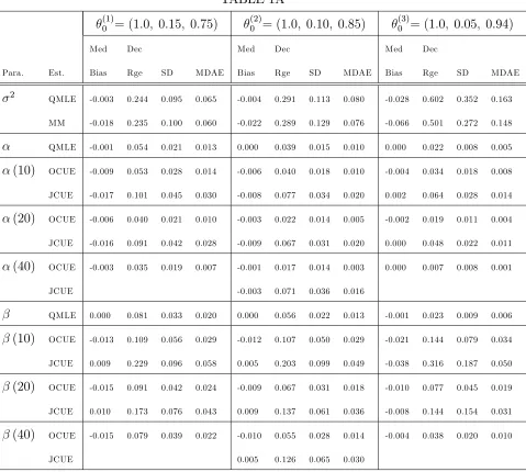
median bias, decile range, and median absolute error are robust measures of central tendency, dispersion, and e¢ciency, respectively, reported out of a concern over the existence of higher moments. The standard deviation, while not a robust measure, provides an indication of outliers. Finally, MM denotes the method of moments plug-in estimator _b2.

Table 1A summarizes the results for the OCUE and JCUE (13 and 19, respectively) at various lag lengthsk, whenmax (i) = 2and = 2. For this speci…cation of _t and the three values of 0 considered, Yt has at least a …nite fourth moment. MM estimates b2 with more

bias than does QMLE, but also with less dispersion. With near uniformity, the dispersion of _b(k) and b(k) for each estimator is decreasing in k. JCUE tends to be less biased than OCUE for b(k), although the magnitudes of the bias for OCUE tend to be small. JCUE is signi…cantly more dispersed than OCUE. The dispersion of _b(k)for OCUE is less than that of _b for k = 20;40. The dispersion of b(k) for OCUE approaches that of b as k increases, exceeding it for (1)0 and

(2)

0 . In these latter two cases, however, the bias of b(k) is higher

than that of b. In summary, when max (i) = 2, OCUE becomes comparable to QMLE ask

increases. JCUE does not.

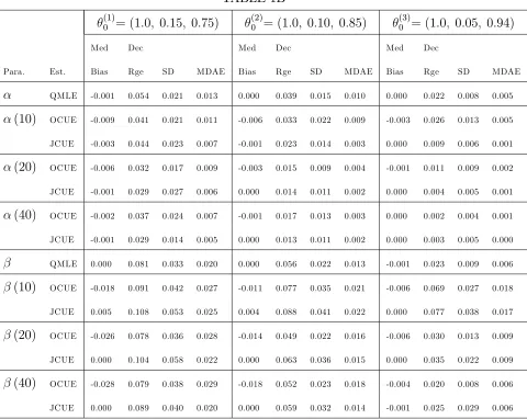
Table 1B summarizes the results for the OCUE and JCUE under the same conditions as Table 1A except thatmax (i) = 3. In this case, for all values of 0 considered, b(k)from the

OCUE is more e¢cient than _b for all k considered. For (3)₀ , b(k) from the OCUE is more e¢cient than b fork = 40. For (1)0 and

(2)

0 , b(k) from the OCUE is less dispersed than b,

but with higher biases. For the JCUE, _b(k)is more e¢cient than_b for allk considered, and

b(k) is seen to approach the e¢ciency of b as k increases. In summary, whenmax (i) = 3, OCUE and JCUE are now seen to both be serious competitors to the QMLE, with the OCUE able to deliver more e¢cient individual point estimates than its QMLE counterpart.

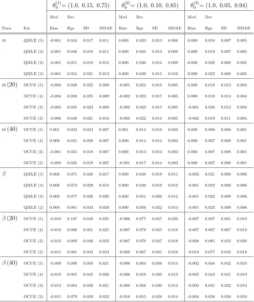
Table 2 summarizes the results for the OCUE at various values of both and k, when

max (i) = 2, for values of 0 considered in the previous tables. Note that higher values of

cases. The dispersion of b(40), on the other hand, is only less dispersed than bwhen = 2. For levels of higher than 2, b(k) is generally more dispersed than b.

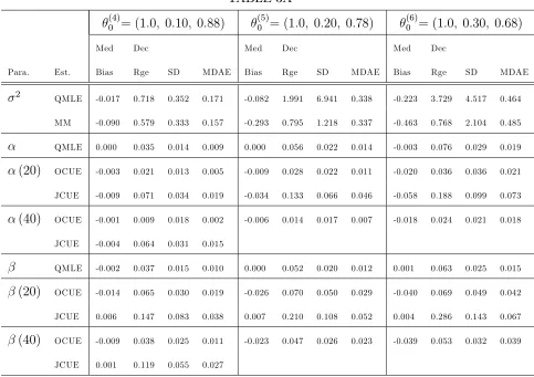
Table 3A summarizes additional simulation results for the OCUE and JCUE when

max (i) = 2, and = 2. In this case, values for ₀ are selected that support a …nite variance of Y_t but not a …nite fourth moment. The degree to which ₀ violates Eh( + 2

t)

2i

< 1

increases from (4)₀ to (6)₀ . In these simulations, neither the QMLE nor the MM estimator is particularly apt at estimating _b2. As before, the QMLE displays relatively less bias but is signi…cantly more dispersed. As expected, JCUE is unbiased for b(k) across the di¤er-ent speci…cations. Unexpected for the JCUE, however, is the …nding that _b(k) evidences non-neglible biases (much larger than those of the OCUE) for speci…cations (5)₀ and (6)₀ . In addition, JCUE is far less e¢cient than the QMLE. Also unexpected is the …nding that OCUE appears to be a serious competitor to the QMLE in the case of (4)₀ . Equally a surprise is the …nding that the OCUE maintains its previous tendency of providing relatively more e¢cient estimates than _b.

Finally, Table 3B replicates the conditions from Table 3A but for max (i) = 3. In this case, a surprising result given the non-existence of the fourth moment is the …nding that both _b(20) and _b(40) for the OCUE and JCUE are more e¢cient than _b for (4)0 and

(5)

0 . Equally surprising for (4)

0 is that the OCUE and JCUE remain serious competitors to

the QMLE generally, since, in each case, b(20) and b(40) are quite comparable to b. In general, for the OCUE and JCUE,b(20) and b(40)tend to be less dispersed than b across the three speci…cations. The biases of b(20) and b(40), however, increase signi…cantly for

(5)

0 and

(6)

0 . While contrary to what theory predicts, the results from Tables 3A and 3B

are supported by simulation results in Kristensen and Linton (2006), where for data lacking a …nite fourth moment, their autocorrelation-based estimator continued to display descent …nite sample performance.

5. FX Spot Returns

-12/31/09 and is obtained from Bloomberg. Consider the spot return de…ned as Y_i;t = log S_i;t=S_{i;t 1} . This section …ts the model of (1) and (2) to Y_i;t T_t=1.14 _{Engle and} Gonzalez-Rivera (1999) as well as Hansen and Lunde (2005) employ similar speci…cations to British Pound and Deutsche Mark exchange rate series, respectively. Hansen and Lunde (2005) …nd no evidence that the simple GARCH(1,1) speci…cation is outperformed by more complicated volatility models in their study of exchange rates. Their work guides the selection of …nancial data analyzed here.

For the AUD series, skewness is 0:33;and kurtosis is15:05. For the JPY series, skewness is 0:43, and kurtosis is 8:34. Both series appear decidedly non-normal with the requisite distributional asymmetry required under A2. Table 4 reports the estimation results for the JCUE, OCUE, and QMLE. For both the JCUE and OCUE, L = 1. For the JCUE, only the speci…cation with max (i) = 3 is considered. For the OCUE, both max (i) = 2 and

max (i) = 3 are considered. Also for the OCUE, when max (i) = 2, k is twice as large as when max (i) = 3 so that the total number of moment conditions being used in each case is the same. Starting values for the JCUE and OCUE are the QMLE estimates.

The JCUE estimates are closer to the QMLE estimates than are the OCUE estimates. For the AUD series, the OCUE with max (i) = 3 implies appreciably higher ARCH and appreciably lower GARCH e¤ects than does the QMLE. For the JPY series, the OCUE with max (i) = 2 produces much larger ARCH and much smaller GARCH estimates than the QMLE. Across both exchange rate series, however, di¤erences in point estimates are accompanied by signi…cantly higher standard errors than in the QMLE case. These higher standard errors are likely related to the near proximity of _b+b to one.

6. Conclusion

The main contribution of this paper is to provide simple GMM estimators for the semi-strong GARCH(1,1) model with a straightforward IV interpretation. The moment conditions from these estimators are stated entirely in terms of covariates observable at timet, and while

14_{Preliminary investigations …t, among other speci…cations, ARMA(1,1) …lters to both series. For the JPY}

they rely on skewness for identi…cation, these estimators do not require treatment of the third and fourth conditional moments. Standard pT-asymptotics apply to these estimators given moment existence criteria no stronger than those required for comparable moment estimators discussed in the literature. These criteria can even be relaxed somewhat by nature of the fact that identi…cation links to properties of the third as opposed to the fourth moment. These simple estimators (can) involve many (potentially weak) moments, the bias from which can be eliminated by using either a CUE with the optimal weighting matrix or what this paper terms the JCUE. Both the OCUE and JCUE can outperform QMLE in …nite samples.

The identi…cation result in this paper can be extended to a GARCH(1,1) model with a leverage e¤ect. Suppose thath_t =!₀+ ₀+ ₀ 1 Y_{t 1} <0 Y2

t 1+ 0ht 1. Then (5) can

be divided into the set of moment conditionsEhYe2

t Yt 1

i

= 0+ 0 P (Yt<0) E[WtYt],

and EhYe2

t Yt 1 1 1 Yt 1 <0

i

= ₀(1 P (Y_t <0))E[W_tY_t], which can be used to identify a semi-parametric IV estimator of the semi-strong GARCH(1,1) model with a lever-age e¤ect. Such an estimator would be applicable to stock returns given the results of Hansen and Lunde (2005) and would expand the set of empirical applications to which simple IV estimators of the GARCH(1,1) model can apply.

Applications in empirical asset pricing involve GARCH assumptions within the GMM paradigm and are, therefore, amendable to the estimators that I propose. For instance, Mark (1988) and Bodurtha and Mark (1991) consider versions of the conditional CAPM that parameterize market betas as ARCH(1) processes. The moment conditions from the simple GMM estimators I propose can easily be appended to the moment conditions of these models to allow the market betas to display GARCH properties without the need for specifying the entire conditional distribution of asset returns.

Appendix

PROOF OF LEMMA 1: From (1) , (2), E W_{t j}z_{t 1} = 0, and the law of iterated

expectations,

EhXe_tY_{t 1}i = Eh eh_t+W_t Y_{t 1}i (21)

= Eh ₀Xe_{t 1}+ ₀eh_{t 1} Y_{t 1}i

= ₀E Y_t3₁ ;

EhXe_tY_{t 2}i = Eheh_tY_{t 2}i

= ₀EhXe_{t 1}Y_{t 2}i

= _{0 0}E Y_t3₂ ;

and

EhXe_tY_{t 3}i = ₀EhXe_{t 1}Y_{t 3}i

= 2₀EhXe_{t 2}Y_{t 3}i

= ₀ 2₀E Y_t3₃ :

Given A2(i), these results imply that

EhXe_tY_{t k}i= ₀ k₀ 1E Y_t3 : (22)

Solving (22) for k=k+ 1 and comparing the result to EhXe_tY_{t k}i produces (6).

LEMMA 2. Given the model of (1) and (2), let Assumptions A1 and A3(i) hold. Then

Eheh2_ti=

2 0

PROOF OF LEMMA 2: Given (4), EhXe2

t

i

=Eheh2

t

i

+E[W2

t]. Given (3),

Eheh2t

i

= 2₀Eheh2t 1

i

+ 2_{0 0}: (24)

Recursive substitution into (24) using (3) produces

Eheh2_ti= 1 + 2₀+ + ₀2( 1) 2_{0 0}+ 2₀ Eheh2_t i

for 1. It is well known that 2_{0 !} 0 as _{! 1} if and only if ₀ < 1, which establishes (23).

PROOF OF THE THEOREM: Given Lemma 2, Y2

t is covariance stationary. As a

con-sequence,_b2 _!p 2

0 by a law of large numbers. Recursive substitution into (8) produces

e

X_t =

1

P

i=0 i

W_{t i}; (25)

where ₀ = 1 and _i = ₀ i₀ 1 for i = 1;2; : : :. Given (25) and A3(i), Ve_t;k is an

L1 _{mixingale (see Andrews 1988 for a de…nition and Hamilton 1994 p. 192-193 for a}

proof). Given A3(ii), T 1P

t

e

V_{t;k !}p 0 (see Theorem 1 of Andrews 1988). Similarly,

e

U_t;k is an L1 _{mixingale given (25) and either A2(ii) or A3(i) for which T} 1P

t

e

V_t;k!p 0

given either A2(iii) or A3(i). It then follows that (a) _bg1;t ;b2 p

! ( 0 ) 0, (b)

b

g₂(k_;t) ;_b2 _!p ₀( ₀ ) k₀ 1 ₀, and (c) _bg₃(k_;t) ;_b2 _!p ( ₀ ) k₀ 1( _{0 0}+ _{0 0}), where g2(k;t) ;b2 and g

(k)

3;t ;b2 are the kth elements of g2;t ;b2 and g3;t ;b2 ,

respectively, for k = 2; : : : ; K and ₀ =Eheh2

t

i

. Let Q( ; 2

0) = g( ; 20)

0

M₀g( ; 2 0),

and Qb ;_b2 =_bg ;_b2 0M_Tbg ;_b2 . Given (a)–(c) and continuity of multiplication,

b

Q ;_b2 _!p Q( ; 2

0). For max (i) = 2, (a) and (b) establish that the only 2

satisfyingg( ; 2

0) = 0is = 0, since 0 6= 0 and 0 is strictly positive. Formax (i) = 3, (a)–(c) establish the same result with parallel reasoning given that _{0 0}+ _{0 0} is also strictly positive. Q( ; 2

0) is then uniquely minimized at = 0. Next, let MT =

LetH b; ; 2

0 =Sb b;b 2 0

M_T Sb ;_b2 , where is betweenb and ₀. Given A5, expanding _bg b;_b2 …rst around ₀, then around 2

0, and then solving for b 0

produces

p

T b ₀ = H b; ; 2 0

1

b

S b;_b2 0M_TpT _bg ₀; 2

0 +Sb 2

0; 2 b2 20

= H ₀; 2

0 1

S ₀; 2 0

0

M₀pT_bg ₀; 2 0 ;

where the second equality follows fromSb b;_b2 _!p S ( ₀; 2

0) given that either Uet;k

is anL1 _{mixingale that is uniformly integrable ifmax (i) = 2orVe}

t;k is anL1 mixingale

that is uniformly integrable if max (i) = 3 and Theorem 1 of Andrews (1988), and

b

S 2 ₀;b

2 p

!0given thatY2

t is covariance stationary. From A4(i) and (25),gt( 0; 20)

is anL2 _mixingale.15 _{Given A6,}p_Tbg(

0; 20)

d

!N 0; ( ₀; 2

0) by Theorem 1 of

De Jong (1997). The conclusion then follows from the Slutzky Theorem.

PROOF OF COROLLARY 1: A4(ii) grants h_t to be -mixing with decreasing mixing coe¢cients (see Corollary 6 of Carrasco and Chen 2002). Theorem 17.0.1 of Meyn and Tweedie (1993) then establishespT_bg( ₀; 2

0)

d

!N 0; ( ₀; 2

0) . The rest follows

from the proof of the Theorem.

PROOF OF THE PROPOSITION: Given the results for derivatives of inverse matri-ces,

@VGM M

@ = 1 2 0 2 0

( 0₀M0 0) 1+ ( 00M0 0) 1 00M0

@ ( 0)

M0 0( 00M0 0) 1 .

15_{The proof of this result follows closely with those of Ue}

t;k and Vet;k being L1 mixingales and is available

Consider …rst the case where ₀ >0, and let x=M0 0( 00M0 0) 1. Then

2

0

( 0₀M0 0) 1+ ( 00M0 0) 1 00M0

@ ( 0)

M0 0( 00M0 0) 1 2

0

( 0₀M0 0) 1+r( 00M0 0) 1 00M0 ( 0)M0 0( 00M0 0) 1 =

r 2

0

( 0₀M0 0) 1 < 0:

Next, consider the case where ₀ <0. Then

2

0

( 0₀M0 0) 1+ ( 00M0 0) 1 00M0

@ ( 0)

M0 0( 00M0 0) 1 2

0

( 0₀M0 0) 1 r( 00M0 0) 1 00M0 ( 0)M0 0( 00M0 0) 1 =

r+ 2 0

( 0₀M0 0) 1 > 0:

PROOF OF LEMMA 3: From the de…nition of_b(_t;sm;n)( ),

b(t;sm;n) b b

(m;n)

t;s ( 0) = 6

T2 ₁ T

1P

t

a_t;s b a_t;s( ₀) :

By the consistency ofbestablished under Theorem 1, ₉a _{t !}0such that b ₀

t. By the triangle inequality,

T 1P

t

a_t;s b a_t;s( ₀) T 1P

t

a_t;s b a_t;s( ₀) T 1P

t t;s

( ) _!p E _t;s( )

PROOF OF COROLLARY 2:

^

Q ;_b2 = T 2

T

P

s=1

T

P

t6=s

g_t ;_b2 0M_Tg_s ;_b2

= T 1

T

P

s=1

T 1

T

P

t6=s

g_t ;_b2 0M_Tg_s ;_b2

= T 1

T

P

s=1

A_s ;_b2 g_s ;_b2 ;

where

A_s ;_b2 = T 1

T

P

t6=s

g_t ;_b2

!0

M_T:

From the Theorem, _bg ;_b2 _!p g( ; 2

0) if max (i) = 2 or 3, which means that each

A_s ;_b2 has the same probability limit. As a consequence, Q^ ;_b2 _!p Q( ; 2 0),

which has a unique minimum at = ₀ (see the proof of the Theorem).

References

[1] Andrews, D.W.K., 1988, Laws of large numbers for dependent non-identically distrib-uted random variables, Econometric Theory, 4, 458-467.

[2] Angrist, J., G. Imbens and A. Kreuger 1999, Jackknife instrumental variables estima-tion, Journal of Applied Econometrics, 14, 57-67.

[3] Baillie, R.T., and H. Chung, 2001, Estimation of GARCH models from the autocorre-lations of the squares of a process, Journal of Time Series Analysis, 22, 631-650.

[4] Bodurtha, J.N. and N.C. Mark, 1991, Testing the CAPM with time-varying risks and returns, Journal of Finance, 46, 1485-1505.

[5] Bollerslev, T., 1986, Generalized autoregressive conditional heteroskedasticity, Journal of Econometrics, 31, 307–327.

[6] Brown, B.W. and W.K. Newey, 2002, Generalized method of moments, e¢cient boot-strapping, and improved inference, Journal of Business and Economic Statistics, 20, 507-571.

[8] Carrasco, M. and X. Chen, 2002, Mixing and moment properties of various GARCH and stochastic volatility models, Econometric Theory, 18, 17-39.

[9] Chamberlain, G., 1982, Multivariate regression models for panel data, Journal of Econo-metrics, 18, 5-46.

[10] Cragg, J.G., 1983, More e¢cient estimation in the presence of heteroskedasticity of unknown form, Econometrica, 51, 751-764.

[11] Donald, S.G., G. Imbens and W.K Newey, 2008, Choosing the number of moments in conditional moment restriction models, MIT working paper.

[12] Donald, S.G., and W.K. Newey, 2000, A jackknife interpretation of the continuous updating estimator, Economic Letters, 67, 239 - 243.

[13] Drost, F.C. and T.E. Nijman, 1993, Temporal aggregation of GARCH processes, Econo-metrica, 61, 909-927.

[14] Engle, R.F., and J. Mezrich, 1996, GARCH for groups, Risk, 9, 36-40.

[15] Escanciano, J.C., 2009, Quasi-maximum likelihood estimation of semi-strong GARCH models, Econometric Theory, 25, 561-570.

[16] Francq, C., L. Horath and J.M. Zakoian, 2009, Merits and drawbacks of variance tar-geting in GARCH models, NBER-NSF Time Series Conference proceedings.

[17] Guo, B. and P.C.B Phillips, 2001, E¢cient estimation of second moment parameters in ARCH models, unpublished manuscript.

[18] Hall, P. and J.L. Horowitz, 1996, Bootstrap critical values for tests based on generalized-method-of-moments estimators, Econometrica, 64, 891-916.

[19] Hamilton, J.D., 1994, Time series analysis, Princeton University Press.

[20] Han, C. and P.C.B. Phillips, 2006, GMM with many moment conditions, Econometrica, 74, 147-192.

[21] Hansen, L.P., 1982, Large sample properties of generalized method of moments estima-tors, Econometrica, 50, 1029-1054.

[22] Hansen, L.P., J. Heaton and A. Yaron, 1996, Finite-sample properties of some alterna-tive GMM estimators, Journal of Business and Economic Statistics, 14, 262-280.

[23] Hansen, P.R. and A. Lunde, 2005, A forecast comparison of volatility models: does anything beat a GARCH(1,1)?, Journal of Applied Econometrics, 20, 873-889.

[25] Kristensen, D. and O. Linton, 2006, A closed-form estimator for the GARCH(1,1)-model, Econometric Theory, 22, 323-327.

[26] Lee, S.W, B.E. Hansen, 1994, Asymptotic theory for the GARCH(1,1) qausi-maximum likelihood estimator, Econometric Theory, 10, 29-52.

[27] Lumsdaine, R.L., 1996, Consistency and asymptotic normality of the quasi-maximum likelihood estimator in IGARCH(1,1) and covariance stationary GARCH(1,1) models, Econometrica, 64, 575-596.

[28] Mark, N.C, 1988, Time-varying betas and risk premia in the pricing of forward foreign exchange contracts, Journal of Financial Economics, 22, 335-354.

[29] Meddahi, N. and E. Renault, 1998, Quadratic M-estimators for ARCH-type processes, working paper CIRANO 98s-29.

[30] Newey, W.K. and D. McFadden, 1994, Large sample estimation and hypothesis testing, in R.F. Engle and D. McFadded, eds, Handbook of Econometrics, Vol. 4, Amsterdam North Holland, chapter 36, 2111-2245.

[31] Newey, W.K. and R.J. Smith, 2004, Higher order properties of GMM and generalized empirical likelihood estimators, Econometrica, 72, 219-255.

[32] Newey, W.K. and D.G. Steigerwald, 1997, Asymptotic bias for quasi-maximum-likelihood estimators in conditional heteroskedasticity models, Econometrica, 65, 587-599.

[33] Newey, W.K and F. Windmeijer, 2009, Generalized method of moments with many weak moment conditions, Econometrica, 77, 687-719.

[34] Pakes, A. and D. Pollard, 1989, Simulation and the asymptotics of optimization esti-mators, Econometrica, 57, 1027-1057.

[35] Schmid, F. and R. Schmidt, 2007, Multivariate extensions of Spearman’s rho and related statistics, Statistics and Probability Letters, 77, 407-416.

[36] Skoglund, J., 2001, A simple e¢cient GMM estimator of GARCH models, unpublished manuscript.

[37] Spearman, C., 1904, The proof and measurement of association between two things, American Journal of Psychology, 15, 72-101.

[38] Stock, J. and J. Wright, 2000, GMM with weak identi…cation, Econometrica, 68, 1055-1096.

[39] Weiss, A.A., 1986, Asymptotic theory for ARCH models: estimation and testing, Econo-metric Theory, 2, 107-131.

TABLE 1A

(1)

0 = (1:0; 0:15; 0:75)

(2)

0 = (1:0; 0:10; 0:85)

(3)

0 = (1:0; 0:05; 0:94)

Med Dec Med Dec Med Dec

Para. Est. Bias Rge SD MDAE Bias Rge SD MDAE Bias Rge SD MDAE

2

QMLE -0.003 0.244 0.095 0.065 -0.004 0.291 0.113 0.080 -0.028 0.602 0.352 0.163

MM -0.018 0.235 0.100 0.060 -0.022 0.289 0.129 0.076 -0.066 0.501 0.272 0.148

QMLE -0.001 0.054 0.021 0.013 0.000 0.039 0.015 0.010 0.000 0.022 0.008 0.005

(10) OCUE -0.009 0.053 0.028 0.014 -0.006 0.040 0.018 0.010 -0.004 0.034 0.018 0.008

JCUE -0.017 0.101 0.045 0.030 -0.008 0.077 0.034 0.020 0.002 0.064 0.028 0.014

(20) OCUE -0.006 0.040 0.021 0.010 -0.003 0.022 0.014 0.005 -0.002 0.019 0.011 0.004

JCUE -0.016 0.091 0.042 0.028 -0.009 0.067 0.031 0.020 0.000 0.048 0.022 0.011

(40) OCUE -0.003 0.035 0.019 0.007 -0.001 0.017 0.014 0.003 0.000 0.007 0.008 0.001

JCUE -0.003 0.071 0.036 0.016

QMLE 0.000 0.081 0.033 0.020 0.000 0.056 0.022 0.013 -0.001 0.023 0.009 0.006

(10) OCUE -0.013 0.109 0.056 0.029 -0.012 0.107 0.050 0.029 -0.021 0.144 0.079 0.034

JCUE 0.009 0.229 0.096 0.058 0.005 0.203 0.099 0.049 -0.038 0.316 0.187 0.050

(20) OCUE -0.015 0.091 0.042 0.024 -0.009 0.067 0.031 0.018 -0.010 0.077 0.045 0.019

JCUE 0.010 0.173 0.076 0.043 0.009 0.137 0.061 0.036 -0.008 0.144 0.154 0.031

(40) OCUE -0.015 0.079 0.039 0.022 -0.010 0.055 0.028 0.014 -0.004 0.038 0.020 0.010

JCUE 0.005 0.126 0.065 0.030

Notes: Simulations are conducted using 5,000 observations across 500 trials. The true parameter vector 0

=( 2

0; 0; 0)0, and = 2. b(k)andb(k)are the and estimates, respectively, based onklags. QMLE

is the quasi-maximum likelihood estimator. MM is the method of moments estimator. OCUE and JCUE are the optimal and jackknife continuous updating estimator, respectively, withmax (i) = 2,k= 10;20;40, and

TABLE 1B

(1)

0 = (1:0; 0:15; 0:75)

(2)

0 = (1:0; 0:10; 0:85)

(3)

0 = (1:0; 0:05; 0:94)

Med Dec Med Dec Med Dec

Para. Est. Bias Rge SD MDAE Bias Rge SD MDAE Bias Rge SD MDAE

QMLE -0.001 0.054 0.021 0.013 0.000 0.039 0.015 0.010 0.000 0.022 0.008 0.005

(10) OCUE -0.009 0.041 0.021 0.011 -0.006 0.033 0.022 0.009 -0.003 0.026 0.013 0.005

JCUE -0.003 0.044 0.023 0.007 -0.001 0.023 0.014 0.003 0.000 0.009 0.006 0.001

(20) OCUE -0.006 0.032 0.017 0.009 -0.003 0.015 0.009 0.004 -0.001 0.011 0.009 0.002

JCUE -0.001 0.029 0.027 0.006 0.000 0.014 0.011 0.002 0.000 0.004 0.005 0.001

(40) OCUE -0.002 0.037 0.024 0.007 -0.001 0.017 0.013 0.003 0.000 0.002 0.004 0.001

JCUE -0.001 0.029 0.014 0.005 0.000 0.013 0.011 0.002 0.000 0.003 0.005 0.000

QMLE 0.000 0.081 0.033 0.020 0.000 0.056 0.022 0.013 -0.001 0.023 0.009 0.006

(10) OCUE -0.018 0.091 0.042 0.027 -0.011 0.077 0.035 0.021 -0.006 0.069 0.027 0.018

JCUE 0.005 0.108 0.053 0.025 0.004 0.088 0.041 0.022 0.000 0.077 0.038 0.017

(20) OCUE -0.026 0.078 0.036 0.028 -0.014 0.049 0.022 0.016 -0.006 0.030 0.013 0.009

JCUE 0.000 0.104 0.058 0.022 0.000 0.063 0.036 0.015 0.000 0.035 0.022 0.009

(40) OCUE -0.028 0.079 0.038 0.029 -0.018 0.052 0.023 0.018 -0.004 0.020 0.008 0.006

JCUE 0.000 0.089 0.040 0.020 0.000 0.059 0.032 0.014 -0.001 0.025 0.029 0.006

Notes: Simulations are conducted using 5,000 observations across 500 trials. The true parameter vector 0

=( 2

0; 0; 0)0, and = 2. b(k)andb(k)are the and estimates, respectively, based onklags. QMLE is

TABLE 2

(1)

0 = (1:0; 0:15; 0:75)

(2)

0 = (1:0; 0:10; 0:85)

(3)

0 = (1:0; 0:05; 0:94)

Med Dec Med Dec Med Dec

Para. Est. Bias Rge SD MDAE Bias Rge SD MDAE Bias Rge SD MDAE

QMLE (5) -0.001 0.044 0.017 0.011 0.000 0.033 0.013 0.008 0.000 0.018 0.007 0.005

QMLE (4) -0.001 0.046 0.018 0.011 0.000 0.034 0.013 0.008 0.000 0.019 0.007 0.005

QMLE (3) -0.001 0.051 0.019 0.012 0.000 0.036 0.014 0.009 0.000 0.020 0.008 0.005

QMLE (2) -0.001 0.054 0.021 0.013 0.000 0.039 0.015 0.010 0.000 0.022 0.008 0.005

(20) OCUE (5) -0.003 0.039 0.025 0.009 -0.001 0.024 0.018 0.005 0.000 0.019 0.013 0.004

OCUE (4) -0.004 0.038 0.025 0.009 -0.002 0.023 0.017 0.005 0.000 0.018 0.014 0.004

OCUE (3) -0.005 0.035 0.023 0.009 -0.002 0.023 0.017 0.005 -0.001 0.020 0.012 0.004

OCUE (2) -0.006 0.040 0.021 0.010 -0.003 0.022 0.014 0.005 -0.002 0.019 0.011 0.004

(40) OCUE (5) 0.001 0.032 0.024 0.007 0.001 0.014 0.018 0.003 0.000 0.008 0.008 0.001

OCUE (4) 0.000 0.031 0.020 0.007 0.000 0.014 0.014 0.003 0.000 0.007 0.009 0.001

OCUE (3) -0.001 0.031 0.018 0.007 0.000 0.013 0.014 0.003 0.000 0.007 0.008 0.001

OCUE (2) -0.003 0.035 0.019 0.007 -0.001 0.017 0.014 0.003 0.000 0.007 0.008 0.001

QMLE (5) 0.000 0.071 0.028 0.017 0.000 0.048 0.019 0.011 -0.002 0.021 0.008 0.006

QMLE (4) 0.000 0.073 0.029 0.018 0.000 0.049 0.019 0.012 -0.001 0.022 0.009 0.006

QMLE (3) 0.000 0.077 0.030 0.020 0.000 0.051 0.020 0.012 -0.001 0.022 0.009 0.006

QMLE (2) 0.000 0.081 0.033 0.020 0.000 0.056 0.022 0.013 -0.001 0.023 0.009 0.006

(20) OCUE (5) -0.010 0.107 0.049 0.025 -0.006 0.077 0.047 0.020 -0.007 0.097 0.081 0.019

OCUE (4) -0.010 0.098 0.051 0.025 -0.007 0.078 0.035 0.018 -0.007 0.067 0.067 0.019

OCUE (3) -0.012 0.089 0.046 0.023 -0.007 0.070 0.037 0.018 -0.008 0.085 0.052 0.020

OCUE (2) -0.015 0.091 0.042 0.024 -0.009 0.067 0.031 0.018 -0.010 0.077 0.045 0.019

(40) OCUE (5) -0.009 0.098 0.050 0.021 -0.006 0.064 0.036 0.014 -0.002 0.048 0.042 0.010

OCUE (4) -0.010 0.085 0.045 0.020 -0.006 0.058 0.030 0.013 -0.002 0.043 0.041 0.010

OCUE (3) -0.012 0.084 0.039 0.021 -0.008 0.056 0.030 0.013 -0.003 0.041 0.022 0.010

OCUE (2) -0.015 0.079 0.039 0.022 -0.010 0.055 0.028 0.014 -0.004 0.038 0.020 0.010

TABLE 3A

(4)

0 = (1:0; 0:10; 0:88)

(5)

0 = (1:0; 0:20; 0:78)

(6)

0 = (1:0; 0:30; 0:68)

Med Dec Med Dec Med Dec

Para. Est. Bias Rge SD MDAE Bias Rge SD MDAE Bias Rge SD MDAE

2

QMLE -0.017 0.718 0.352 0.171 -0.082 1.991 6.941 0.338 -0.223 3.729 4.517 0.464

MM -0.090 0.579 0.333 0.157 -0.293 0.795 1.218 0.337 -0.463 0.768 2.104 0.485

QMLE 0.000 0.035 0.014 0.009 0.000 0.056 0.022 0.014 -0.003 0.076 0.029 0.019

(20) OCUE -0.003 0.021 0.013 0.005 -0.009 0.028 0.022 0.011 -0.020 0.036 0.036 0.021

JCUE -0.009 0.071 0.034 0.019 -0.034 0.133 0.066 0.046 -0.058 0.188 0.099 0.073

(40) OCUE -0.001 0.009 0.018 0.002 -0.006 0.014 0.017 0.007 -0.018 0.024 0.021 0.018

JCUE -0.004 0.064 0.031 0.015

QMLE -0.002 0.037 0.015 0.010 0.000 0.052 0.020 0.012 0.001 0.063 0.025 0.015

(20) OCUE -0.014 0.065 0.030 0.019 -0.026 0.070 0.050 0.029 -0.040 0.069 0.049 0.042

JCUE 0.006 0.147 0.083 0.038 0.007 0.210 0.108 0.052 0.004 0.286 0.143 0.067

(40) OCUE -0.009 0.038 0.025 0.011 -0.023 0.047 0.026 0.023 -0.039 0.053 0.032 0.039

JCUE 0.001 0.119 0.055 0.027

Notes: Simulations are conducted using 5,000 observations across 500 trials. The true parameter vector

0 = ( 2

0; 0; 0)0, and = 2. b(k) and b(k) are the and estimates, respectively, based onklags.

TABLE 3B

(4)

0 = (1:0; 0:10; 0:88)

(5)

0 = (1:0; 0:20; 0:78)

(6)

0 = (1:0; 0:30; 0:68)

Med Dec Med Dec Med Dec

Para. Est. Bias Rge SD MDAE Bias Rge SD MDAE Bias Rge SD MDAE

QMLE 0.000 0.035 0.014 0.009 0.000 0.056 0.022 0.014 -0.003 0.076 0.029 0.019

(20) OCUE -0.002 0.008 0.008 0.003 -0.008 0.014 0.017 0.008 -0.020 0.024 0.016 0.021

JCUE -0.001 0.007 0.008 0.001 -0.006 0.022 0.017 0.006 -0.018 0.049 0.030 0.018

(40) OCUE -0.001 0.004 0.005 0.001 -0.007 0.011 0.016 0.007 -0.020 0.022 0.012 0.020

JCUE

QMLE -0.002 0.037 0.015 0.010 0.000 0.052 0.020 0.012 0.001 0.063 0.025 0.015

(20) OCUE -0.011 0.036 0.016 0.012 -0.026 0.042 0.022 0.026 -0.042 0.051 0.025 0.042

JCUE -0.004 0.039 0.020 0.009 -0.018 0.048 0.043 0.019 -0.031 0.085 0.057 0.032

(40) OCUE -0.011 0.027 0.012 0.012 -0.023 0.047 0.026 0.023 -0.045 0.053 0.023 0.045

JCUE

Notes: Simulations are conducted using 5,000 observations across 500 trials. The true parameter vector 0

=( 2

0; 0; 0)0, and = 2. b(k)andb(k)are the and estimates, respectively, based onklags. QMLE is

TABLE 4

Currency Para. JCUE OCUE QMLE

max (i) 3 2 3

k 40 80 40

b2 0.5579 0.5579 0.5579 0.4957

b 0.0511 0.0706 0.1192 0.0532

AUD (0.0979) (0.0608) (0.0088)

b 0.9215 0.9180 0.8772 0.9382

(0.0276) (0.0231) (0.0101)

b+b 0.9726 0.9887 0.9964 0.9914

max (i) 3 2 3

k 40 80 40

b2 0.4963 0.4963 0.4963 0.5057

b 0.0539 0.1984 0.0558 0.0486

JPY (0.0517) (0.0443) (0.0095)

b 0.9099 0.7523 0.9277 0.9361

(0.0288) (0.0114) (0.0123)

b+b 0.9638 0.9507 0.9835 0.9848

Notes: GARCH(1,1) models are …t to Australian Dollar (AUD) and Japanese Yen (JPY) spot returns, where the spot rates are measured in terms of US Dollars. The time period for each series is daily from 1/1/90 - 12/31/09. JCUE and OCUE are the jackknife and optimal continuous updating estimator, respectively, where

L= 1. kis the number of lags used in the given estimator (if applicable). max(i)speci…es whether the given estimator is based on properties of the third moment only (max(i) = 2) or also on properties of the fourth (max(i) = 3). b2