An image reconstruction algorithm for a dual modality tomographic system

(1)

An image reconstruction algorithm for a dual modality

tomographic system.

NORDIN, Md. Jan.

Available from Sheffield Hallam University Research Archive (SHURA) at:

http://shura.shu.ac.uk/20268/

This document is the author deposited version. You are advised to consult the publisher's version if you wish to cite from it.

Published version

NORDIN, Md. Jan. (1995). An image reconstruction algorithm for a dual modality tomographic system. Doctoral, Sheffield Hallam University (United Kingdom)..

Copyright and re-use policy

(2)

SHEFFIELD HALL AM UNIVERSITY LIBRARY CITY CAMPUS POND STREET

SHEFFIELD 31 1WB

1 0 1 4 4 1 9 8 6 7

&Wo<ai-Sheffield Hallam University

(3)

ProQuest Number: 10700913

INFORMATION TO ALL USERS

The quality of this reproduction is dependent upon the quality of the copy submitted.

In the unlikely event that the author did not send a com plete manuscript and there are missing pages, these will be noted. Also, if material had to be removed,

a note will indicate the deletion.

uest

ProQuest 10700913

Published by ProQuest LLC(2017). Copyright of the Dissertation is held by the Author.

This work is protected against unauthorized copying under Title 17, United States C ode Microform Edition © ProQuest LLC.

ProQuest LLC.

789 East Eisenhower Parkway P.O. Box 1346

(4)

An Image Reconstruction Algorithm for a

Dual Modality Tomographic System

by

Md Jan Nordin

BSc MSc

A thesis submitted to

Sheffield Hallam University

for the degree of Doctor of Philosophy

in the School of Engineering Information Technology

(5)

Acknowledgements

I would like to record my sincere thanks to my main supervisor, Professor Bob Green, for his intelligent supervision, helpful suggestions and constructive criticisms of my work. I am extremely grateful for his outstanding support and encouragement throughout the course of this research. >

I would also like to express my sincere thanks to my co-supervisors, Dr Ivan Basarab and Dr Fraser Dickin (Process Tomography Unit, UMIST) for their help and advice.

For my colleagues in Room 2302 School of Engineering Information Technology, Tony, Ruzairi, Fuad, Neil, Marshall and Joe, thank you for your valuable discussions and suggestions.

(6)

Dedication

(7)

Abstract

This thesis describes an investigation into the use of dual modality tomography to measure component concentrations within a cross-section. The benefits and limitations of using dual modality compared with single modality are investigated and discussed. A number of methods are available to provide imaging systems for process tomography applications and seven imaging techniques are reviewed. Two modalities of tomography were chosen for investigation {i.e. Electrical Impedance Tomography (EIT) and optical tomography) and the proposed dual modality system is presented. Image reconstruction algorithms for EIT (based on modified Newton-Raphson method), optical tomography (based on back-projection method) and with both modalities combined together to produce a single tomographic imaging system are described, enabling comparisons to be made between the individual and combined modalities.

To analyse the performance of the image reconstruction algorithms used in the EIT, optical tomography and dual modality investigations, a sequence of reconstructions using a series of phantoms is performed on a simulated vessel. Results from two distinct cases are presented, a) simulation of a vertical pipe in which the cross-section is filled with liquid or liquid and objects being imaged and b) simulation of a horizontal pipe where the conveying liquid level may vary from pipe full down to 14% of liquid. A computer simulation of an EIT imaging system based on a 16 electrode sensor array is used. The quantitative images obtained from simulated reconstruction are compared in term of percentage area with the actual cross-section of the model. It is shown from the results that useful reconstructions may be obtained with widely differing levels of liquid, despite the limitations in accuracy of the reconstructions.

The test results obtained using the phantoms with optical tomography, based on two projections each of sixteen views, show that the images produced agree closely on a quantitative basis with the physical models. The accuracy of the optical reconstructions, neglecting the effects of aliasing due to only two projections, is much higher than for the EIT reconstructions. Neglecting aliasing, the measured accuracies range from 0.1% to 0.8% for the pipe filled with water. For the sewer condition, i.e.

(8)

1. Introduction

This chapter introduces the idea of using tomographic imaging for monitoring individual components of multi-component flows. The aim of the project was to measure the volume flow rates of major components of sewage. Single modality tomography systems have proved effective in the monitoring of dual component flows such as liquid/gas, liquid/solid etc., but are inadequate when more components are present. Therefore, in this work two modalities of tomography were chosen for investigation {i.e. Electrical Impedance Tomography (EIT) and optical tomography). The work reported in this thesis concentrates on the investigation of image reconstruction for EIT, optical and with both modalities combined together to produce a single tomographic imaging system for sewers.

1.1 An overview of process tomography

The need for tomographic imaging in the process industry is analogous in many respects to the medical need for clinical diagnostic purposes (Dickin et al., 1992a). The general principle underlying process tomography is to attach a number of non- intrusive sensors (transducers) in a plane or a number of planes of the vessel to be studied. Unlike medical tomography, which has been successful by the development of computer assisted tomography (CAT) (Herman, 1980), the development of tomographic instruments for process applications are still undergoing development (Isaksen, 1994). The main reason for this is the difficulty in designing an instrument which is robust and operable in aggressive and fast moving environments such as multicomponent flows which are common in process applications.

(12)

handling multicomponent flows by enabling boundaries between different components in a process to be imaged (Dickin et al., 1992a) and, if necessary, in real-time (Cook and Dickin, 1993). The resultant tomographic images should therefore yield a representation of the internal structure of the process vessel in two-dimensions (Dickin

et al., 1992a). These images can be used for example in identification of individual components in multicomponent flows. With this form of information more readily available, process 'diagnosis' becomes more accurate and consequently more precise guidance can be given for monitoring and control purposes (Dickin et ah, 1992b).

Potential applications of process tomography to industrial-based equipment are limited. However, of particular interest in environmental monitoring is the investigation of volume flow rates of the major components of sewage - this being the application described in this project. The use of conventional measuring instruments, such as those based on optical techniques as a means of acquiring measurement information, is severely limited in most practical conditions since, some of the components inside the sewers exhibits a high degree of opacity. On the other hand, the use of electrical-based tomography does not suffer this limitation since it depends on the electrical properties of the multicomponent flows. However, if these techniques

(i.e. EIT and optical measurements) combine together and form a dual modality tomographic imaging system, there is a possibility more information can be acquired than with a single modality system.

The main components of sewage are cellulose material (papers, rags, etc.), rubbers, plastics, solids and conveying liquid (mainly water based). Each has varying physical properties making them difficult to detect using a single measurement technique. For instance, if the flow is dominated by non-conducting materials (i.e.

(13)

1.2 The aims and objectives of the thesis

The main aim of the work reported in this thesis is to investigate the feasibility of applying a dual modality (resistive electrical impedance tomography and optical tomography) system to map multicomponent flow for the measurement of volume flows in sewers. This leads to a challenging image reconstruction problem, that is to combine data from both techniques to produce single dual modality tomographic images. This requires superimposing the two images obtained from the two types of sensors. The sensing principles are difficult; EIT is a soft field method, while optical sensors are line sensors and also they detect different materials (some materials may be transparent to one type of sensor). The aims can be stated in more detail as follows:

1. To study the fundamental principles of electrical impedance tomography and optical tomography and to investigate the feasibility of using them for process- based application.

2. To study the performance and limitations of existing medical-based image reconstruction methods, to implement and, if necessary, to modify and further develop these methods for use on multi-component flows.

3. To visualise multi-component flow mixtures by mapping the cross-section inside the pipe.

4. To study the reconstructed images for a range of materials within a liquid conveyor in terms of image 'quality* and range of materials detected.

5. To establish the accuracy and limitations of the dual modality system by testing it with simulated data using numerical approaches.

(14)

1.3 Organisation of the thesis

Chapter 1 of this Thesis presents a brief introductory description on the topic of process tomography. The aims and research objectives are described, followed by a brief description of the Thesis structure.

Chapter 2 reviews the imaging techniques. A number of methods are available to provide imaging systems for process tomography applications, of which some are discussed in this chapter.

Dual modality imaging system for sewers is described in Chapter 3. This chapter introduces the idea of using tomographic imaging for the monitoring of volume flows of the various components in sewers.

The principles of image reconstruction method are introduced and reviewed in Chapter 4. This chapter consists of three major parts. In the first the image reconstruction method for an electrical impedance tomography system is described. In the second the image reconstruction method for the optical imaging system is described. The final part describes how both techniques can be combined to produce a single dual modality tomographic image.

Chapter 5 presents results from numerical simulated data for EIT. This chapter analyses the results obtained from the EIT image reconstruction method and compares them using quantitative measure.

(15)

Chapter 7 presents results from numerical simulated data for dual modality. This chapter analyses the results obtained from combining both EIT and optical tomography system for the monitoring of concentration profiles of the various components in sewers. The results are compared and analysed using a quantitative measure.

(16)

2. Imaging Techniques

A number of methods are available to provide imaging systems for process tomography applications, of which some are discussed in this chapter.

2.1 Positron Emission Tomography (PET)

Positron emission tomography is based upon the distribution of activity of positron emitters. Radioactive carriers or emitters are injected into the process to be studied. A function of position and time in relation to the emitters is obtained from external coincidence measurements. The fundamental measurement is the coincidence detection of two almost anti-parallel photons, which are emitted as a result of the annihilation of a positron with an electron. Imaging systems involve either circular geometry, with rings of sensors around the flow to be imaged, or position sensitive detectors, such as gamma cameras or multiwire proportion chambers (Parker et al.,

1992).

(17)

2.2 X-ray

X-ray transmission computed tomography is one of the main imaging techniques used in diagnostic medicine. It was through its success at solving medical imaging problems that it was chosen to be applied in other areas such as engineering.

Two kinds of X-ray imaging are X-ray transmission radiography and X-ray transmission tomography (Simon, 1975). For X-ray transmission radiography, the image is static. It is the shadow of the object formed by a transmitted X-ray impinging on a detector such as photographic film. This is not a desirable method where flow imaging is concerned, as it provides no method of providing a continuous image of the flow.

In X-ray transmission tomography, the concern is with the provision of images of sections or thin slices through an object at different depths. This is achieved by the carefully calculated and controlled relative motion of the X-ray source and the detector during the exposure. This technique has become known as computerised tomography,

(i.e. a CT scan). The equipment needed for this is large and bulky, and a high element of danger is involved due to the presence of ionising radiation (Simon, 1975) — so this is not the best suited tomographic tool for flow imaging in an industrial setting.

2.3 Nuclear Magnetic Resonance (NMR)

(18)

When a nucleus with spin is placed in a magnetic field, it will attempt to line up with the field. With a quantum number I = 1/2, the nucleus can take up one of two stable states - namely parallel to the field, or the opposite direction. These correspond to high and low energy states, but there will be a bias to the lower energy state, as given by Bolzmanns equation:

^=-=exp(/j/7yfcr)

NUP

Where N^own, NUp are the number of nuclei with spin up and spin down, k is Bolzmanns constant, h is Planck's constant and T is the absolute temperature.

In this aligned state, the sample will achieve a net magnetisation, which is the quantity observed in NMR, and is proportional to the applied field - so a higher applied field gives a greater sensivity. The applied magnetic field is provided by an RF magnetic field pulse generator, and the received signal is a weak, free induction signal emanating from the subject. The actual image obtained is of proton density within the subject. This is a very expensive way of imaging which would not be viable for imaging flows at present. Extensive work on Magnetic Resonance Imaging (MRT) using modified nuclear magnetic resonance (NMR) systems is being performed at Cambridge University and in the USA (Dickin et al., 1992b).

2.4 Ultrasound

(19)

The equipment in ultrasound measurements include an ultrasonic generator, a transducer to transmit and receive ultrasonic waves, and some kind of computerised image processing system. A technique known as Doppler ultrasound (Kremkau, 1990) is used to image a moving interface. An interface is the boundary region between two different objects, or types of tissue. The ultrasonic signal is strongly reflected wherever there is an interface between one tissue and another - allowing a degree of localisation and discrimination which is not possible with X-ray images. When the ultrasonic waves strike the moving interface, the frequency of the reflected waves is altered in proportion to the velocity of the moving interface. This technique can be used to visualise flow in blood vessels throughout the body (Jaffe, 1984). However, there is some danger present when using ultrasound. Ultrasound exposure of a bone/tissue interface can result in sudden and sometimes pronounced periosteal pain arising from a build-up of heat at the interface (WHO, 1982; Lehmann et al., 1967).

Ultrasound is now being applied to flow imaging in pipes, and research is being undertaken to develop a tomographic system for flow imaging with ultrasound. Work on ultrasound sensing has been carried out to measure bubble velocities in two phase flow (Xu et al., 1988). The ultrasonic transducer is excited using extremely short duration voltage pulses which causes a pulse of energy to propagate through the flow medium. The propagated pulses are attenuated by a magnitude dependent on the properties of the materials contained within the flow. The signal received at the detector is a train of amplitude modulated pulses which can be processed and low pass filtered to produce an analogue wave form. Investigations by Pinkard (1990) for the Water Research Council suggested that the use of ultrasonics to detect solids within sewage flows was impractical due to the lack of contrast between the attenuation properties of the conveying liquid and solid material such as faeces. In addition, it has been shown (Beyer and Letcher, 1969; Muir and Carstensen, 1980; Carstensen et al.,

(20)

2.5 Capacitive impedance tomography

Electrical capacitance tomography is based on the principle that the movement of materials through the sensing volume will alter the permittivity and hence the measured capacitance of the volume. A number of electrodes are mounted circumferentially around a pipe, and the capacitance between all combinations of electrode pairs measured. The dielectric distribution within the pipe is usually reconstructed using the Linear Back Projection (LBP) method (Xie et al., 1992). At present, a capacitive tomography system for imaging pipelines containing insulating mixtures (such as solids/gas and liquid/gas) is already delivering images of powder/air and kerosene/nitrogen flows (Dickin et al., 1992b). It uses a charge-transfer capacitance transducer working at 15 volts with a noise level as low as 0.08 r.m.s and a 6" pipeline twelve-electrode system (Huang et al., 1992; Xie et al., 1992). It enables void fraction and the flow regime to be determined and is the first key stage in developing a non-invasive two-component mass flow meter.

However, according to (Isaksen and Nordtvedt, 1992) accurate quantitative information from such a system is difficult to obtain due to the following problems: a) Ho simple relation between the measured capacitance and the dielectric

distribution exists.

b) The electric field between the source and detector electrodes determine the sensitive region, which does not posses a sharp boundary.

c) The sensitivity for the measured quantities is not constant within the sensitivity region.

(21)

2.6 Electrical Impedance Tomography (EIT)

Electrical Impedance Tomography (EIT) is concerned with obtaining images of •bodies' by non intrusive means. Electrodes are placed around the subject and signals are fed onto-into the body, the remaining electrodes are used to take voltage readings. These readings are fed into a computer which processes the information into the form of a conductivity/resistivity map. The conductivity/resistivity map is displayed on the computer screen. The map is colour coded to highlight areas of equal conductivity/resistivity. It is used, for example, in medicine to take cross sectional studies of arms, legs, breasts and the torso (Bhat, 1990). This will be discussed in more detail in Section 3.2.

2.7 Optical Tomography

(22)

2.8 Discussion

(23)

3. Dual Modality Imaging System (DMIS)

for Sewers

In this chapter an outline of the proposed dual modality system is presented. The chapter consists of three sections. The first and second sections deal with the EIT imaging system and the optical imaging system respectively. The last section is a description of how both technologies are combined to investigate dual modality tomography.

3.1 Introduction

Electrical Impedance Tomography (EIT) is a method for revealing the internal structure of a conducting object or a living body without destruction by reconstructing an image that represents the space distributed property of the materials it contains. The main application of image reconstruction is in medicine, with computerised tomography, which allows one to analyse the structure of human organs, detect tumours, and aid medical diagnosis (Jossinet et al, 1988; Eyuboglu and Brown, 1988; McArdle et al., 1988). Applications of EIT in the process industry are new although these applications are growing very quickly as industry appreciates their use (Xie et al.,

1994; McKee et al., 1994).

Image reconstruction can help to visualise multi-phase flow distributions and the distribution of the components in a variety of systems, for example, oil pipelines and sewers. This flow information is not only important under steady operation but also under transient and fault conditions.

(24)

characteristics of the main constituents of sewage, a combination of two or more detection methods will need to be used. For this project, based on a literature search on the most applicable work, data from two detection methods is investigated. This results in dual modality tomographic imaging, which in this case is based upon electrical impedance tomography (Webster, 1990; Gisser et al., 1987; Samakato et al.,

1987; Yorkey, 1986 and Abdullah, 1993) and infra-red matrix imaging (Saeed et al.,

1988; Dugdale et al., 1992 and Dugdale, 1994).

The three major solid components of sewage to be detected are rubber, effluent solids and cellulose products. Rubber should be detectable by impedance methods while solids should be visible to an infra-red matrix system. The main problem comes with any cellulose products where a low resistivity is expected, due to the absorption of fluids, and its translucency under these conditions is unknown.

3.2 Electrical Impedance Tomography System

The objective of electrical impedance tomography is to produce an image which correctly represents the impedance characteristics of a region of interest. In doing so it is important to have some idea of the system's ability .to provide a quantitative representation of those impedance characteristics.

The strategy used in the present work for measuring the voltages at the periphery of the pipe is called the neighbouring method. A pair of adjacent electrodes is selected and a current is applied between them. The potential gradients established between the rest of the pairs of adjacent electrodes are measured. This sequence is repeated until all the adjacent pairs have been selected for current injection and the corresponding boundary voltage gradients have been measured. For a system with

N electrodes, using the 4 electrode measurement method, a total of N*(N-3)/2

(25)

The finished system should be able, to distinguish a solid from a liquid from a gas, as sewerage pipe flows will almost always contain multicomponent flows. The images to be produced do not have to be as high in resolution as normally needed for medical imaging, only the order of the size and distribution of each component of the flow, in a cross-section, are required.

cross-section through vessel

display unit data acquisition

system

image reconstruction system

sensor electrodes on vessels

Figure 3.1 A typical EIT system

A typical EIT system is shown in Figure 3.1. It consists of three subsystems described in the following subsections:

a) sensor subsystem

b) data acquisition system (DAS) c) image reconstruction and display

3.2.1 Sensor subsystem

(26)

number of constraints on the sensors. Ideally it should be compact, non-intrusive, require minimum maintenance or calibration, and in many cases be intrinsically safe. The electrodes are usually mounted on the surface around the object. The number of electrodes used depends on the complexity and resolution of the images required. The number of electrodes used at present is typically 16, 32 or 64.

3.2.2 Data acquisition system (DAS)

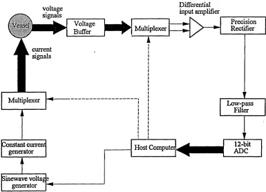
Due to the constraints imposed by the strict safety requirements of clinical instruments the majority of biomedical DAS's are restricted in the range of measurements they can make. DAS for the process industry do not have this restriction (except in safety critical situations) and can therefore have a much wider dynamic measurement range. Currents injected into the object are provided by voltage controlled current generators. Many current injection methods have been proposed by EIT investigators (Webster, 1990) such as: adjacent, opposite, multireference, multisink and optimal. The injection method has a significant effect on the quality of the images produced (Webster, 1990). For accurate voltage measurements the injected currents amplitude must be maintained constant throughout the measurement period. This requires current and voltage generators with very good stability and low harmonic distortion (Wang et al., 1992).

(27)

voltage signals Differential input amplifier Multiplexer

I

Voltage Buffer current signals Multiplexer Host Computer Precision Rectifier Constant current generator Low-pass Filter 12-bit ADC

[image:27.621.75.460.55.333.2]

Sinewave voltag 3 generator

Figure 3.2 Components of typical EIT data acquisition system

3.2.3 Image reconstruction and display

Voltages measured by the data acquisition system (DAS) are passed to the image reconstruction algorithm. This algorithm uses the voltages taken from a number of independent measurements to map the resistivity distribution of the object’s cross- section. For N electrodes (for the four-electrode measurement method) there are N(N- 3)/2 independent measurements (Seagar, et al., 1987).

(28)

inverse problem which determines the resistivity distribution given only the boundary current conditions. In essence, a reconstruction algorithm first makes an initial guess of the resistivity distribution. It then uses the forward problem solver to calculate the boundary voltages. These voltages are compared with the DAS measured voltages. Errors formed by the calculated and measured voltages are used to update the resistivity distribution. This process is repeated until the error between the forward problem solver and the measured values reach a predefined level. Generally, the inverse problem requires the solution of the forward problem.

From the point of view of the reconstruction of resistivity distribution images and neglecting problems associated with data collection accuracy is dependent on several factors including:

a) accuracy of the forward problem solver b) accuracy of DAS

c) effectiveness of the reconstruction algorithm

A special problem that the image reconstruction must take into consideration for this project is the depth of the conveying liquid, which will vary. All existing tomographic imaging systems have a priori knowledge of the process boundary.

Different algorithms for reconstruction have been proposed by many researchers. Each method has its merits and limitations. Yorkey et al., (1990) provides a good reference on the effectiveness of various reconstruction algorithms used in EIT. The main methods currently being used are:

• fast filtered back projection method (Barber and Seagar, 1987) and (Seagar et al, 1987).

• iterative equipotential lines method (Yorkey et al, 1987).

• perturbation method (Kim et al, 1987) and (Yorkey et al, 1987). • double constraint method (Wexler et al, 1985)

(29)

3.3 Optical Imaging System

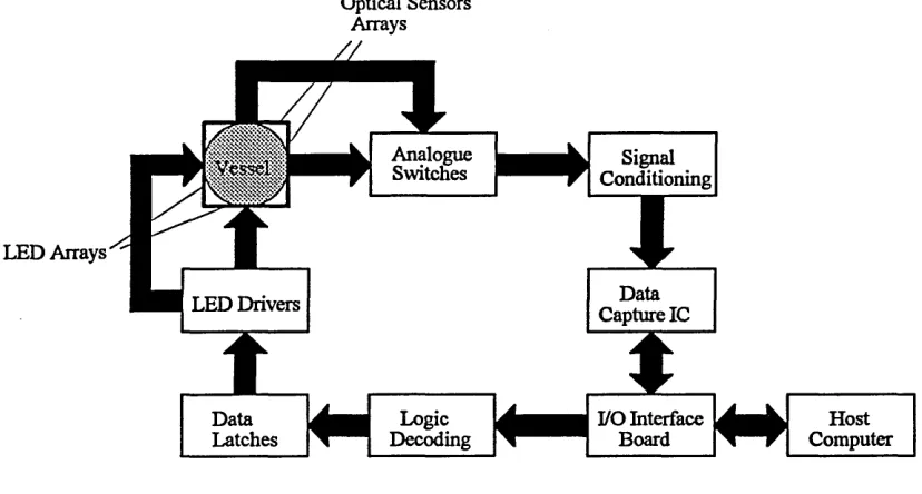
Optical Tomography involves projecting a pencil of light through some medium from one boundary point and detecting the level of light received at another boundary point. This single pencil of light is called a view. The principle is straight forward, as light travels through space it suffers attenuation for a variety of reasons, such as scattering and absorption. Different materials cause different levels of optical attenuation and this fact forms the basis of optical tomography. Several pencils of light are used in parallel to produce one projection. This procedure provides information from which a profile of the flow can be gained. In practise several projections are required to minimise aliasing which occurs when two particles intercept the same view. This process is described by Saeed et ah, 1988, where two component flows are monitored.

(30)

Optical Sensors Arrays

LED Arrays

Signal Conditioning Analogue

Switches

1

Data Capture IC LED Drivers

t

Logic

Decoding I/O InterfaceBoard Data

[image:30.616.83.497.34.256.2]

Latches ComputerHost

Figure 3.3 Schematic diagram of an optical tomography system

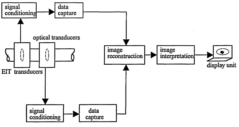
3.4 The Data Collection System

The basic system shown in Figure 3.4 below uses two different arrays of transducers. The transducers, one optical the other EIT, are being investigated to determine if they are capable of identifying the main constituents of the sewers. Both EIT and optical sensors are mounted on the same section of the pipe. The EIT system uses 16 electrodes and is capable of injecting a constant current via any two electrodes and measuring the resultant voltage differentials produced at any other two electrodes. The optical hardware is designed around two projections of 16 transducer pairs as this allows basic image reconstruction to be applied to the acquired data.

(31)

optical transducers

display unit EIT transducers

data capture signal

conditioning

data capture signal

conditioning

image interpretation image

[image:31.616.84.495.27.245.2]

reconstruction

Figure 3.4 The proposed dual modality imaging system for sewers

(32)

[image:32.612.174.350.31.204.2]

imm&m

(33)

4. Image Reconstruction Method

In this chapter theory relating to the reconstruction of tomographic images is presented. The chapter is divided into three sections. The first and second sections deal with image reconstruction methods for EIT systems and image reconstruction methods for optical imaging systems respectively. The final section is a description of how tomographic images from both techniques can be manipulated to produce single tomographic images of volume concentrations of multicomponents in a test section.

4.1 Image reconstruction method for EIT system

The task of image reconstruction in electrical impedance tomography can be divided into two distinct parts (Section 3.2.3):

(a) the forward problem (b) the inverse problem.

4.1.1 The forward problem

(34)

For a simple two-dimensional model such as the cross-section of a circular process vessel, the solution to the forward problem can be analysed using an analytical solver even though numerical techniques such as the finite element method (FEM) are preferred (Webster, 1990). The preference for the latter is due, in part, to the fact that the FEM is more flexible in handling problems involving a vessel with a complicated geometrical shape and accommodating inhomogeneous material distributions within it. The conductivity/resistivity distribution within the region is partitioned into discrete elements each with assumed constant conductivity/resistivity. By exploiting continuity of voltage and current flow at the boundaries of the elements the problem is reduced to the solution of a generally large series of linear equations. Murai and Kagawa (1985) model the finite element method as a discrete resistance network, equivalent to assuming that within an element the voltage is a linear function of position. Dines and Lytle (1981) also use a simulated resistance network, though not one equivalent to a finite element model, and solved the forward problem by a systematic application of the Kirchhoff currents laws to the nodes of the network.

4.1.1.1 Mathematical preliminaries

(35)

potential inside the object through which a steady state alternating current is flowing can be derived from a combination of Maxwell's electrostatic equations given by

V*(cV<|)) = 0 in r (4.1)

where a is the conductivity of the medium and <j) is the electrical flux. The object, which in this case is a process vessel, is represented by the symbol T and II is given to represent its boundary. Also, collectively referred to as the Laplace equation, the

reference, in this situation, to three-dimensional Cartesian co-ordinates (x,y,z) :

Like any other boundary value problem, the partial differential equation shown in equation (4.1) can subsequently be solved by applying the appropriate boundary conditions. In EIT, alternating current is applied through one pair of electrodes and the resulting voltages measured through a different pair of electrodes attached to the object's boundary (this is referred to as the adjacent measurement technique). Hence, the equivalent boundary conditions associated with applying currents are of the Neumann type given by:

differential vector operator V in equation (4.1) specifies the space differentiation with

(4.2)

(4.3)

on the negative driving electrode and,

(4.4)

(36)

(4.5)

In practice the voltages are not completely determined until a reference condition is specified. One convenient way of achieving this is:

N

5>/=o

(4-6)

/=i

In this manner, equation (4.1) together with the conditions in equations (4.3), (4.4) and (4.6) can be solved to yield a unique set of solutions (Cheney and Isaacson, 1991). Hence the forward problem can be diagramatically stated as:

► find von II

Figure 4.1 The forward problem in EIT

In the following sub-sections, mathematical procedures based on the finite element method are outlined for general two and three-dimensional cases even though, for simplicity, a two-dimensional case was implemented and used throughout this study. Lnven a (conducuvity)

along with boundary and reference conditions

forward problem

4.I.1.2 Finite element modelling (FEM) of a typical process vessel

(37)

a completely homogeneous state. However, in many cases the process medium exhibits complex impedance inhomogeneity and under this condition direct integration is not possible. Instead, a piece-wise approximation can be employed which is based on the finite element method. This forms part of the motivation for using the FEM throughout this research for modelling and theoretical studies.

Application of the FEM to the solution of a physical problem is based on the minimisation of energy. Employing variational calculus, the solution to equation (4.1) and its associated boundary conditions is identical to finding a function <}> which minimises the functional %:

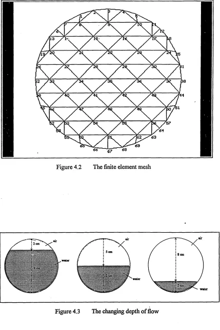
From equation (4.8) integration is carried out over the whole domain T and <j) must be a continuous function possessing the piece-wise continuous first derivatives of the domain T (Zienkiewicz and Cheung, 1965). In order to implement equation (4.8) the domain is divided into m individual finite elements forming a mesh. For a cylindrical shaped domain the most popular (and most straightforward to implement) types of elements considered are triangular and quadrilateral shaped elements. The former is used to discretize the whole domain in this project. An example of the FEM mesh used in this study is shown in Figure 4.2

(38)

by functional Ai(x,y,z)</>j, A2(x,y,z) <t>2, —, A s(x,y,z)<j)s respectively, then <j>^ can

be treated as a linear combination of the above functions i.e.

4 e) (x,y,z) = Ai(x, y, z) <f>j+A2( x, y, z)#2+--+As( x, y, z) </>s (4.9)

or,

(41°)

k=l

In this case the field variables ^ represent the model potential of each element and s

its node number. Equation (4.10) can be written in matrix form to yield:

/ = M M (4.11)

(39)

From equation (4.12) for the ith node:

dfa dx d<j>\dx,J dy d<j>\ dy * dz d(j>{ \dz*

+ \ \ \ j ^ r dxdydz = 0

n ^

'dxdydz

(4.13)

Substituting equation (4.11) into equation (4.13) gives:

g f A

HH

+

dA\ dA.2

dc ’ ck dx dh\ SSji dA

dy ’ dy dy

J

+

dA,

J£' L

dz ' & ' ' £ JJJy(A/)<iw?y<fe = 0

n

(4.14)

For the entire element, equation (4.13) can be written in matrix form:

Yj> = c (4.15)

(40)

and,

'dz

(4.16)

d= - j j j j A,dafydz (4.17)

n

Assuming that the interpolation functions A/ for modelling the behaviour of <|> satisfy the compatibility and completeness requirements, the final equation for minimising the functional % can be derived by assembling and summing the contributions to a typical differential i. e.

where m is the total number of elements chosen in the domain, and the superscript (e)

denotes an element. Furthermore, for a particular node z, only the values of (j) at those nodes connected to it will appear and their coefficients will involve only the contributions from elements adjacent to the this node. This arrangement produces a typical 'narrow-band' set of simultaneous equations (Abdullah et al., 1992) which can be written same as equation (4.15), where Y is a square matrix whose coefficients are determined from the geometrical co-ordinates of element vertices and from the element conductivities; <j) is the column vector corresponding to the number of unknown values and, in this case, the nodal potential; c represents the boundaiy currents. Hence, the general field problem given in equation (4.1) has been transformed into a set of algebraic equations which can be solved by a variety of techniques such as the Cholesky factorisation method described in more detail latter.

In this study, only a two-dimensional FEM solution is implemented even though its extension to three-dimensional problems would be relatively straightforward

m

z = Z z (e)t (e) (4.18)

(41)

(see Suggestion for future work, Section 8.3). Hence, the representative field equation in the two-dimensional case can be simplified to give:

A { a * £ \ + A { a £ £ ) s o

Scy Sc) ty y dy) (4.19)

The equivalent function to be minimised reduces to:

•jMf)+£r(^)

■dxdy+\\j‘fdxdy

(4.20)

The design of the mesh texture to implement equation (4.1) warrants further explanation. It is often desirable to predict nodal potentials to the highest possible precision. This can be achieved using the smallest size elements possible particularly in the most sensitive part of the vessel. In EIT, the most sensitive part is the region in vicinity of the vessel's boundary. Hence, it is worthwhile placing as many finite elements as possible at the vessel's boundary region. However, the total number of elements forming the mesh is limited by the number of independent measurements available from the data collection system. For instance, if the number of. elements is larger than the total number of independent measurements, the inverse problem will be under-determined. This effect is quite undesirable in many quantitative reconstruction algorithms such as the MNR algorithm since, for the under-determined system, there are more unknowns than equations and consequently, there is either no solution or an infinite number of solutions (Yorkey, 1986). Thus, to implement the MNR the chosen number of elements, in the mesh must satisfy the condition specified below (Yorkey,

1986):

Number of elements in the mesh <M= ——

(42)

where N is the number of electrodes. However, at present, the adjacent measurement method is employed which further reduces M and hence the number of elements in the mesh to (Yorkey, 1986):

N ( N -3)

Number of elements in the mesh < M - —^ — - (4.22)

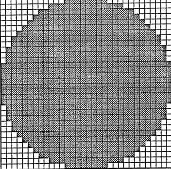
For a 16-electrode system i.e. N = 16, the number of independent measurements is 104. Thus, to ensure that the reconstruction problem is always determined {i.e. the number of unknowns must at least be equal to the number of equations), the number of elements chosen was exactly 104. The arrangement of the 104 elements inside the mesh is shown in Figure 4.2, where there are 69 nodes which are numbered.

(43)

13

12

57

69 69

[image:43.619.68.497.32.673.2]

66

Figure 4.2 The finite element mesh

(44)

It can also be seen from Figure 4.2 that the size of elements used in the mesh are relatively large. As a result, an accurate approximation (i.e. less than 1% error) of the field distribution inside the domain is difficult to attain. For example, as mentioned in the above paragraph, there is a steep gradient in the field intensity from the regions near the vessel boundary to its central axis. Thus, a finer mesh structure is desirable in these regions to accommodate the above phenomena. However, this configuration is only practical provided there are a sufficiently large number of independent measurements, i.e. N = 32 or more. Clearly for a 16-electrode system, the design of the finite element mesh is limited as evidenced in Figure 4.2 which leads to image reconstruction problems. These problems are due to extreme ill-conditioning of the Hessian matrix (Yorkey, 1986) which consequently requires the use of a regularisation technique to force the MNR algorithm to converge towards a solution.

4.1.1.3 Formulation of the forward problem.

Consider the region in which the problem to be solved is divided into triangular elements (one of them is shown in Figure 4.4 below). Also, let the triangle be defined by nodes 1, 2 and 3 and their respective local co-ordinates (xi,}^), (^2^ 2) ^

(*3,^3) respectively.

x

(45)

The set of function <j>, constrained to be a set of first order polynomials for each triangle whose value at any point within the triangle, is a linear interpolation of the vertex values such that:

(f*) = cci + a2x + ayy (4.23)

For all three nodal conditions this leads to a system of equations:

(4e) = “ 1 + “2*1 + “3^1

4 e) = ax + a2x2 + a- ^ 2 (4.24)

4 ^ = «i + a2x2 + a3y3

Solving for a\, a i and 0 3 from equation (4.24) and substituting these values into

equation (4.23) gives:

(4-25>

where, _j

An = 2 '^e) (Qn+bnx+cny) n - 1, 2, 3 (4.26)

also,

^ (e) = area of triangle 1,2,3 a i=X2y3-x3y2

b\ — y 2~y3 (4.27)

Cl = X3 -X 2

the other coefficients (a2,a3,b2,b3,c2,c3) can be obtained through a cyclic

(46)

£k 2 A bn ” 1 , 2 , 3

1 , 2 , 3

Substituting equation (4.28) into equation (4.16) gives:

Yy - 4 A ( e ) 2

JJ

(bi b j+a cj)dxdy for/,7 = 1, 2,3

Noting that:

jjdxdy = A,t>

Equation (4.29) becomes:

^ =

-jibihj+vcj) for i,j= 1, 2, 3

For the whole element, Y can be written in matrix form:

Y =

b2 + c2 b2bj + c2Cj bjbj + c3c2

b2bj 4* CjCj b2 4* c2 bjb2 + c3c

bjbj+CsCj bjb2 +c3c2 b3 4-c

Since the region has been divided into p triangular elements, the complete representation of the field variable (j) over the whole domain is given by:

n=l n-l

(4.28)

(4.29)

(4.30)

(4.31)

(4.32)

(47)

Finally, the assembly of element equations to obtain the system equations for all the domain follows the standard method given by (Huebner, 1975) can be written the same as equation (4.15), where Fis a n x n sized matrix having units of conductance (units: Siemen), <j> is a n xl sized vector which represents the voltage vector at n discrete points inside and on the boundary of the mesh, c is also is a n x 1 sized vector which

has units of amperes and contains the applied currents at n points on the boundary. In order to solve uniquely equation (4.15), a reference condition is specified by grounding the central node inside the mesh shown in Figure 4.2. This is done by setting all entries in the ith column and row corresponding to the reference node to zero and setting its diagonal element to unity. Matrix F, historically referred to as the stiffness matrix, has several properties. First, it is symmetrical and very sparse. Second, matrix Fis a positive definite matrix. Third, Fis also double centred, i.e. the sum total of the elements in any given column or row is zero. These properties of F resemble those of a classical admittance matrix (Mitra, 1969).

4.1.1.4 Classical method of solving = c

Since F is a symmetric positive definite matrix it has a unique Cholesky factorisation given by:

Y = LLr (4.34)

where L is a real non-singular lower triangular matrix with positive diagonal elements. The Cholesky factorisation algorithm used to compute Jy is given by:

jt-i

/„ = J'if-Z /iU for i= 1 , 2 n (4.35)

(48)

Consequently, the solution of equation (4.15) is obtained by solving two triangular systems:

Forward substitution: Z = £ _1c (4.37)

Back substitution: Z (4.38)

Since there arep current projections, i.e. ci,C2 ,'”>Cp, their corresponding solutions,

i.e. are obtained by repeatedly multiplying Y~l with each current

projection. The final solution is re-arranged to give an p x I sized dimensional vector:

(4-39)

Since the potential difference measured at each receiving electrode is required a transformation matrix T is introduced into equation (4.39) to give:

v = T<j> (4.40)

(49)

Read mesh file

i

Construct matrix Y

FindY

Enter boundary conditions

Solve Y c

---Yes _{i = i+}1

(next projection)

Form forward vector v

[image:49.619.144.424.51.531.2]

stop

Figure 4.5 Flow chart for the forward solver

4.1.2 Inverse Problem

(50)

conducting objects inside the process vessel from a set of measured boundary voltages. This procedure is referred to as the inverse problem in EIT. The conductivity/resistivity imaging problem is the inverse of the forward problem and involves the determination of the distribution of conductivity/resistivity within the region from voltage measurements at the surface of the object. For the forward problem specification of the surface current distribution and the conductivity/resistivity distribution it is sufficient to determine the distribution of the voltage within the object. However, a set of surface voltage measurements derived from a single applied current distribution does not carry enough information to uniquely solve for the conductivity/resistivity distribution except under highly constrained conditions. In order to calculate the conductivity/resistivity distribution several independent sets of measurements are needed. Given a set of applied current patterns and their associated surface voltage measurements the inverse problem becomes one of finding a conductivity/resistivity distribution which is consistent with the measurements and any particular constraints that can be applied to the problem. The relationship between the conductivity/resistivity distribution and the surface voltage distribution is a non-linear one and this is bound to present some extra difficulties with the inversion.

The solution of the inverse problem in EIT is not straightforward since the relationship between v and p(x,y), where p the resistivity is 1/conductivity, is highly

non-linear. As such the solution of the inverse problem to produce quantified results, highly desirable for validating process models, generally requires an iterative (multi- step) solver. In an iterative solver, such as the regularised Newton method (Breckon and Pidcock, 1988), the reconstruction process commences with an initial 'predicted* resistivity distribution and uses this to solve the forward problem thereby producing calculated boundary voltages. These calculated voltages are compared to their measured counterparts to produce an 'error1 or difference factor which is subsequently

(51)

pre-defined tolerance. In this work the iterative reconstruction algorithm is used. The iterative algorithm is based on the modified Newton-Raphson method.

4.1.2.1 Modified Newton-Raphson (MNR) method

One of the most theoretically orientated iterative reconstruction algorithms developed for image reconstruction in electrical impedance tomography is that based on Yorkey's resistor network (Yorkey, 1986). Using computer simulated data, Yorkey demonstrates the superiority of the MNR algorithm compared to other reconstruction techniques such as the backprojection method (Barber et al, 1983), the perturbation method (Kim et al, 1983) and the double-constraint method (Wexler et al, 1985). Biomedical EIT investigators such as the RPI group in the USA and the Sheffield University group have not adopted the MNR algorithm for reconstruction because of its convergence problems (Yorkey, 1987). In contrast, Yorkey's colleagues at Wisconsin University reported limited success in applying this algorithm to medical applications, in particular visualisation of the human lung (Woo et al, 1992).

The FEM is introduced as a standard tool to solve, what is in effect, a boundary value problem. In essence, the FEM replaces the distributed Laplace equation with a set of linear algebraic equations which are solved to form an n

dimensional vector v. This vector contains n independent data sets from a mesh containing ^ ’boundary electrodes and p projection angles. The vector v can be written as follows:

(52)

1 < i < p

for i + 2 < k < N - 1, i = 1

7 + 2 <k< N, i& l

(4.42)

In equation (4.41) denotes the differential voltage measured between the k

and k + Ith electrodes resulting from a current applied between i and / + Ith pair. In order to obtain a complete set of independent measurements, p current patterns are applied and their corresponding boundary voltages calculated. These voltages are 'stacked' to form an n dimensional column vector denoted by vcal while its equivalent sized measured counterparts are denoted by vmea. Following a standard least-squares technique the sum squared difference between vcal and vmea is found which is referred to as the objective function cp (Abdullah et al., 1992). Thus:

1 T

~ [^ca/

Hence, an optimal solution to the non-linear inverse problem corresponds to the minimum value of (p. To obtain the minimum (p equation (4.43) is differentiated with respect to each variable in vf 1 and the final result equated to zero. Thus:

? ’ = [% ,] = o (4.44)

where the matrix is given by:

r . I (4.45)

L dps

(53)

The Taylor series expansion of equation (4.44) yields:

<p'(p )= <p{p)+ <p'{p){p-p) (4.46)

The second order derivative <p appearing in the RHS of equation (4.46) is known as the Hessian matrix H and evaluation of all its entries is one of the most computationally intensive procedures encountered in the MNR-based inverse solver. Moreover, the contribution of the last term in the RHS of equation (4.46) is small and hence, to make considerable economies in computation, the Hessian matrix is approximated to:

ff=?V)

= [v„,]r [v„,] (4.47)

By substituting equations (4.47) and (4.44) into equation (4.46) and setting the latter to zero gives:

[Vla(f[V~l - ] +[Vl«/]r[Vl<,1]A/ =

0 (448)

where (p-p*) is denoted as Apk. Equation (4.48) can be re-arranged to produce the

desired updating equation shown below:

^ = ~ {[v« '] r [v« ']} [v~i]r [v«rf-v„*a] (4-49)

The first derivative v ^ , is also referred to as Jacobian matrix J and it is given by:

(54)

Equation (4.51) is the 'standard' method of forming J despite the availability of alternative methods such as those based on the compensation theorem (Yorkey, 1990). As mentioned by Yorkey, even though the compensation method is more efficient in computing J it is only suitable when the measuring technique is that of the adjacent pairs. In contrast, the standard method offers more flexibility because it can be applied to any measurement technique. Therefore, the standard method was used in this work to form the Jacobian matrix.

The MNR algorithm eventually iterates into a minimum (representing the final solution) using the update equation given in equation (4.49). At the kth iterative step the element vector is updated by:

=f/c+ A ff (4.52)

(55)

predicted resistivity distribution which is nearly the same as the true value of the conveying liquid inside the pipe was used to overcome the problems.

In the next section the image reconstruction method for the optical system is outlined.

4.2 Image reconstruction method for optical imaging system

In this work visible light is used to replace X-rays for the scanning of multi phase flow as suggested by (Dugdale, 1994, Hartley et. al., 1991 and Dugdale et. al,

1991). In infra-red transmission systems radiation follows a similar attenuation law to X-rays when the beams cross an air-water system. The laws governing light are complex, but if certain approximations are made, they can be simplified. For the purpose of a simple reconstruction algorithm it is assumed that the beams of light travel in straight lines. In the next sub-section the theory of the method used, which is based on the principle of optical attenuation, is described

4.2.1 Mathematical preliminaries

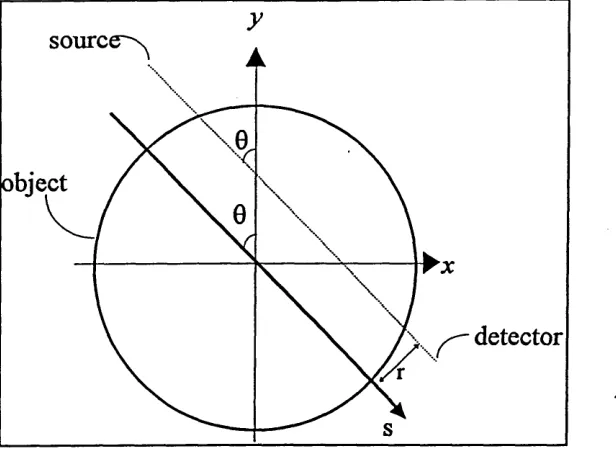
The rectangular co-ordinate system (x,y) is used to describe any point in the layer under examination (Fig. 4.6). The linear attenuation coefficient fi, is used to describe a property of an object as a whole. The optical density function J(x,y),

(56)

) s o u rc e ^

\

b

xN

object / \

k

\ _\

\

_\

\ \

V \ _N W v_{I ^} \ \ I

A ^ detector

— s

Figure 4.6 Co-ordinate systems. Points within the object are described by a fixed (x,y) co-ordinate system. Rays (dashed line) are specified by their angle with respect to the j-axis, 0 and their distance from the origin, r. The s co-ordinate denotes distance along the ray.

A straight line from the source to the detector, which the path of the radiation follows, is termed the ray-path and is described by an (r,s) co-ordinate system which is rotated by the same angle as the ray. Each ray is thus represented by a polar coordinate system (r,Q)y where r is the distance from the origin and 0 is the angle of the ray with respect to the y-axis. Thus, the line integral of the attenuation coefficient,

fix,y) is given by

p(r,6) = jf( x ,y ) d s (4.53)

r.0

where p(r,Q) is the linear attenuation coefficient along the ray path, at distance r from the origin, and angle 0 to the y-axis. Now for optical radiation

[image:56.621.141.449.33.261.2]

(57)

where / 0 = original intensity of source

I = measured intensity

|x = linear attenuation coefficient

x ~ thickness of object

In the following analysis the effects of reflection and refraction are neglected. Only optical attenuation is considered. Then

I = I0exp(amdm) (4.55)

where I is the light intensity after a distance dm, 70 is the initial light intensity and am

is the attenuation constant of the medium through which the light is travelling. Therefore, for a constant distance across a circular pipe and a constant light intensity the received light strength is a function of the average attenuation coefficient over the path length.

4.2.2 Image reconstruction for optical tomography

(58)

Measurements of light intensity passing through an object at a certain cross- section make it possible to calculate its internal distribution of optical density. The reconstruction problem is stated as follows: estimate from a finite number of projections the density distribution in the section of the original object. The principle of measurement acquisition is shown in Figure 4.7.

object to be reconstructed

Figure 4.7 Acquisition of the projections

(59)

Rty k

Figure 4.8 The square pixels model for transmission tomography image reconstruction.

Thus

(4-56) j=i

i = 1, 2,..., n for each ray,

where Pk is the ray sum of the Ath ray (/. e. ray attenuation), at is the value of the ith pixel, and wik is a geometric factor corresponding to the effect of the £th ray on the zth pixel; it is zero if the ray does not pass through the pixel. The image reconstruction problem is to determine the pixel values aJt a2 an from the set of ray sums Pk. This work attempts to use the back-projection method because it is straight forward and the optical data is limited to two projections in this system.

4.2.2.1 Back Projection Method

(60)

the receiver position. The ray-sum values at the receivers are back projected to light intensity values in the area between the two overlapping lines as shown in Figure 4.9.

light detector

J m

view line

m k light

detector light

source

f m

view line

light source

Figure 4.9 Overlapping pixels for two view lines

The density for each point in the reconstructed image is obtained by summing up the densities of all the rays which pass through that point. Reconstruction is performed by back-projecting each profile across the plane i.e. the magnitude of each ray-sum is applied to all points that make up the ray. The process may be described by the equation

f(x ,y ) = ^ ”=lp(xcos0+ys\n 0)A0 (4.57)

(61)

where 0 = is theyth projection angle

A0 = is the angular distance between projections and the summation extends over all the m projections

f(x ,y ) is only used to emphasise that the density values are not equivalent to the true densities f

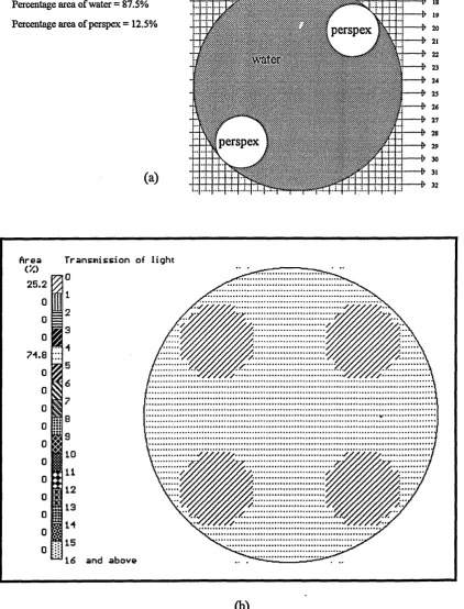
Therefore for a constant distance across a circular pipe and a constant initial light intensity, the final light intensity measured at the receivers can be obtained by summing up all the pixel values of all the rays which pass through the sensing path as shown in Figure 4.10. Hence, for the limited data provided by the two projections, the whole of the pipe cross section, which is represented by 16x16 squares, can be obtained by superimposing the sensitivity paths produced by each projection.

(62)

light detectors

7 8 9 10 11 12 13 14 15 16

'•'W

^4{'V ,< :4 \ mum

K i$ + N j+ i-t-S

a

w<?y

I I _&v§

cNvw

£H+ ^ 1W>M

light detectors

phantom

light sources

Figure 4.10 The square model that was used for optical measurements

(63)

BEGIN

Read input values for all views REPEAT

Check if ray sum for this view represents water

IF represent water, indicate all pixels for this view as water pixels UNTIL end of view (i.e 32 views)

REPEAT

Check if pixel j in this view is water pixel

IF water pixel THEN accumulate temporary ray sum ELSE increment counter for pixel not water

store the position of j UNTIL (j > 16)

Assign all pixels that are not water =

(measured ray sum - temporary ray sum) / total pixels not water UNTIL end of projection (i.e 2 projections)

(64)

start

Yes

No

Yes _{i <= 32 ?}

No view[i] = water

increment i get input file

32 views

initialise i =1

assign all pixels for this view as water pixels

(65)

initialise 1 =1

initialise temp ray sum

initialise counter not water = 0

initialise j =1

ixel[i j] = wate

increment not water counter

accumulate temp ray sum

store position not water pixel (i.ej)

increment j

for not_water pixel = measured ray sum - temp ray sum

not water counter

view end ?

rejection end

Yes

(66)

4.3 Dual modality tomography image reconstruction

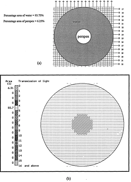
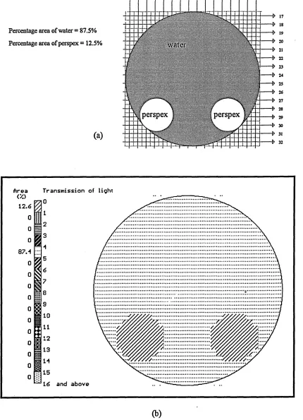
Dual modality tomography images are produced by superimposing images obtained by both EIT and optical measurements (Figure 4.12). Tomographic images from EIT use a range of colours to represent pixel resistivity and tomographic images from optical measurements use a range of patterns to represent optical transmissivity. When both tomographic images are superimposed the final image is a combination of colours and patterns. Both techniques display an image based on a 16x16 array. From these colours and patterns various properties with respect to conductivity/resistivity and translucence to light can be obtained. A set of results produced by superimposing these two techniques are discussed more detail in Chapter 7.

Optical images

superimposing both images

Dual modality images

(67)

For the optical part of the dual modality reconstruction algorithm, the pixel values representing the light intensity, which are displayed by patterns on the screen, are stored in an array OPT(32, 32). The information concerning the resistivity values, which are represented by colours, are stored in another array EIT(32, 32). The OPT data has better resolution but the reconstructions suffer from aliasing. The EIT data is less accurate, but does not suffer from aliasing.

(68)

Figure 4.13

No OPT[i,j] = me;

for optical dati

Yes No Yes j <=32? iNo Yes i<=32? ,No stop start increment j increment i initialise j =1 initialise i =1