The development of a Wireless Sensor Network sensing node utilising adaptive self diagnostics

The development of a Wireless Sensor Network

sensing node utilising adaptive self-diagnostics.

Hai Li1

, Mark C. Price12

, Jonathan Stott1

, and Ian W. Marshall1

1 _{Computing Laboratory, University of Kent, Canterbury, UK, CT2 7NF.}

2 _{School of Physical Sciences, University of Kent, Canterbury, UK, CT2 7NH.}

[email protected]

Abstract. In Wireless Sensor Network (WSN) applications, sensor nodes are often deployed in harsh environments. Routine maintenance, fault detection and correction is difficult, infrequent and expensive. Further-more, for long-term deployments in excess of a year, a node’s limited power supply tightly constrains the amount of processing power and long-range communication available.

In order to support the long-term autonomous behaviour of a WSN system, a self-diagnostic algorithm implemented on the sensor nodes is needed for sensor fault detection. This algorithm has to be robust, so that sensors are not misdiagnosed as faulty to ensure that data loss is kept to a minimum, and it has to be light-weight, so that it can run continuously on a low power microprocessor for the full deployment period. Addition-ally, it has to be self-adapative so that any long-term degradation of sensors is monitored and the self-diagnostic algorithm can continuously revise its own rules to accomodate for this degradation. This paper de-scribes the development, testing and implementation of a heuristically determined, robust, self-diagnostic algorithm that achieves these goals.

1

Introduction

1.1 Background: The PROSEN project.

PROSEN (PROactive condition monitoring of SEnsor Networks) is an EPSRC funded, multi-university project [1] which is investigating techniques to enable automated control and proactive management of sensor arrays. The project aims to develop a proactive Wireless Sensor Network (WSN) to enable condition mon-itoring of a wind farm in an uncontrolled, unsupervised, outdoor environment that will be deployed for a minimum of one year.

policy rules which can be modified on individual nodes. For example, an event could be generated when a sensor records a measurement above (or below) a certain (policy determined) threshold, when a possible sensor fault is detected, or when the battery voltage of the node reaches a certain critical level.

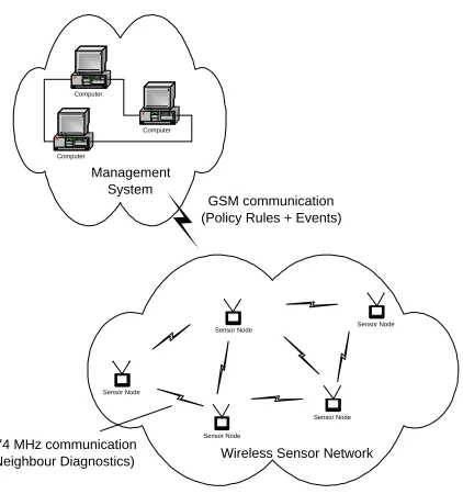
Figure 1 is a schematic showing the information flow within the PROSEN WSN. Each node will also have a short range (174 MHz) radio in order to commu-nicate with its nearest neighbour. This enables a second level of data verification if, for example, one node is measuring an abnormally high temperature, it can query its neighbour to verify the validity of the reading. If the sensor reading is invalid then a possible sensor fault condition is flagged, and reported to the management system.

Computer

Computer

Computer

Management System

GSM communication (Policy Rules + Events)

Sensor Node

Sensor Node

Sensor Node

Sensor Node

Sensor Node

174 MHz communication

(Neighbour Diagnostics) Wireless Sensor Network

Fig. 1.Schematic showing information flow within the PROSEN WSN.

In traditional condition monitoring systems, the sensor nodes acquire data under the control of a local microcontroller located on the node, and then raw data is transmitted to a central base-station (e.g. PC). This central base-station then performs high level, CPU intensive, functions such as data analysis and decision making (e.g. [2]).

To tackle the drawbacks of such a system, we are investigating and demon-strating techniques that enable the automated control and management of sensor arrays to be proactive. In order to achieve this goal, we need to give the sensor nodes much more on-board ‘intelligence’ such as self-diagnosis, data analysis, asessment of data quality and decision making routines.

The obvious challenge with such an approach, is that it requires a sophis-ticated processor on each node to handle the data analysis, self-diagnosis and decision making processes. Such processing power comes at the expensive of in-creased power useage, thus further constraining the frequency and duration of power hungry, long-range communications. There is therefore a requirement to develop a self-diagnostic algorithm that is not only robust and adaptable, but will run on a low power microprocessor.

1.2 Approaches to sensor self-diagnosis.

Automated fault detection techniques have been widely studied and developed during the last few years (for example, Angeli et al. [3]) and the most popular methods include model-based methods [4, 5] and artificial intelligence methods [6]. These methods are highly reliable and are robust, but all are based on highly complicated computation, thus requiring a high speed processor, large amounts of memory, and therefore have a high power consumption. Two further examples are Nithyset al.[7] and Farinazet al.[8].

Nithyset al. [7] developed a cross-validation based technique for on-line de-tection of sensor faults. Their idea is to compare the results of multisensor fusion with, and without, each of the sensors involved using non-linear function min-imization and then identify the faulty sensor using non-parametric statistical techniques. Their simulation results indicate the high accuracy of the approach, but the implementation complexity of non-linear function minimization is too high for a low power microprocessor with limited memory and processing speed. Farinazet al.[8] propose a distributed, localized, sensor fault detection al-gorithm for WSNs. In their alal-gorithm, each node monitors its health status and that of its nearest neighbours. This data is correlated and exchanged be-tween the nodes. Each node therefore has knowledge of its own status and all its neighbours. The drawback of this algorithm is that there is a large amount of information transferred between nodes, resulting in a high power overhead due to the wireless communications required.

A further avenue is to use a rule-based approach. Betrand-Krajewskiet al. [9] present a formal approach to the establishment of a such a rule-based system. The major advantage which such a system is the low processing power required, and the rapidity in which a working rule-set can be tested, evaluated, modified and retested.

example, such a directive could be:“If measurements from a sensor are identified as noisy, either check the battery or the connectors on the sensor and to the sensor-board”. Their approach is a high level fault detection technique running on the base station side, but requires a large amount of node-human interaction to quickly identify, then remedy problems.

In this paper, we describe and evaluate a light weight heuristically determined rule-based algorithm to identify possible sensor faults for each of our sensor nodes. It has a low computing complexity and (so far) has achieved a 100% sucess rate in detecting faults, with no false-positives reported.

We describe the architecture of our prototype platform in Section 2. Sec-tion 3 describes our low level self-diagnosis routines, and presents some practical results, and Section 4 gives conclusions and future work.

1.3 Hardware development strategy.

From the outset, our design strategy has been to minimise the duration and frequency of long range communications, and limit such communications to the transmission of events (ie. alarms, alerts, node health status etc.), and the re-ception of policy rules which determine the conditions under which these events are generated.

We therefore adopted the following methodology:

1. Deploy a “first generation” prototype node in a controlled external envi-ronment to measure base-line operational parameters of the sensors and communications components. This has a simple self-diagnostic rule set, and event generating capability.

2. Develop a “second generation” node that will have full system functional-ity. This will have an adaptive self-diagnostic rule-set, full event generating capability and be able to receive updates from the management system. It will also incorporate two processors, a low power micro-processor that per-forms low-level tasks, and a higher power processor which is powered up intermittently to perform more CPU intensive tasks.

3. Using data from the first and second generation nodes, fully optimise the hardware architecture and system parameters for the finalised “third gener-ation” node to maximise the node lifetime.

2

A prototype sensor node

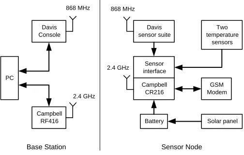
MHz RF transmitter and receiver. We also integrated a Campbell Scientific CR216 wireless datalogger [12], which has five 12-bit analogue inputs, two pulse inputs, two digitial I/O lines, a RS-232 port and a RF416 spread spectrum radio (operating at 2.4 GHz) so that we can monitor the sensors in parallel with the Davis ISS (via the custom built sensor interface) [13]. This logger has a user-programmable 8-bit microprocessor with 6.5 KBytes of program space, and 250 KBytes of data storage, and it is on this platform we have implemented our data acquisition and self-diagnosis algorithm for our first generation node.

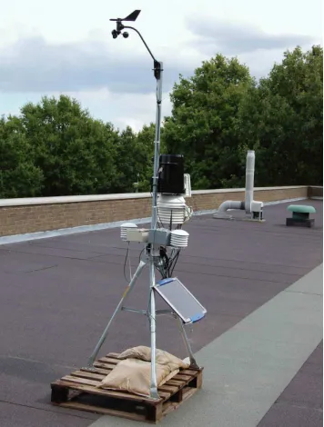
Figure 2 shows the various components of the node. The “Base Station” side is located within the School of Physical Sciences building at the University of Kent, and the “Sensor Node” is deployed on the first floor roof of the same building (Figure 3). Initial deployment was carried out in July 2006.

Davis sensor suite

Sensor interface Campbell CR216

GSM Modem

Two temperature

sensors

Battery Solar panel 868 MHz

2.4 GHz

Sensor Node

Davis Console

Campbell RF416 PC

868 MHz

2.4 GHz

Base Station

Fig. 2.Components of our first generation prototype node.

In addition we have also connected the Campbell data logger to a GSM modem via its RS-232 interface. This allows us to send events and alarms to a remote system via SMS. This has proved to be very effective, felixble and reliable and will be developed into a two-way process in our second generation node [14].

As we also anticipate that the time between battery replacements in the field could be anywhere between one and two years, we have added a 0.18 m2

Fig. 3.A photograph of the deployed first generation sensor node.

3

Self-Diagnostic methods

3.1 Establishing the initial rule-set.

To establish an effective rule set, we used heuristic, phenomenological and sta-tistical methods to establish:

1. Sanity levels. This is simply a set of values based upon possible non-physical readings, ie. a humidity reading greater than 100% (or less than 0%), tem-peratures less that -40o

centigrade, or greater than +40o

centigrade etc. Any reading outside of these values is a probable sensor malfunction.

2. Maximum and minimum environmental parameters (ie temperature, humid-ity, wind speed) over a long period. This was achieved by analysing a data set from a nominally identical weather station that has been deployed for two years within a mile of our prototype node [15], plus additional data ob-tained from the met office [16]. Any deviation of the measured values outside of these values could be indicative of a sensor fault.

3. Noise parameters. Specifically the standard deviation of the noise of a sensor over a long period. Again, any increase (or decrease) in these values may suggest a sensor problem.

be strongly correlated, and any deviation from this correlation could be characteristic of a malfunction in either sensor.

In order to illustrate our methodology, we now discuss three examples of how we obtained our base-line performance parameters for the temperature sensors, the solar radiation sensor and the anemometer.

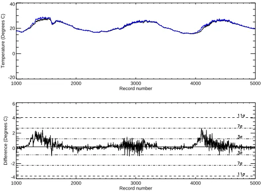
We have installed two Campbell Scientific (Model 109) temperature sensors on our prototype node. They are housed within their own radiation shields and are approximately 1 metre from the floor with a horizontal separation of 25 cm. In Figure 4 (top) we have plotted the temperature as measured by our two temperature sensors for a three day period, and (bottom) the residuals between the two readings.

In order to calculate a base-line noise value, we calculated the standard de-viation, σ, of the residuals for 50,000 readings (equivalent to 33 days of data), also plotted on the bottom graph of Figure 4 are the±3, 7 and 11σ levels.

As these temperature sensors are nominally identical, in the absence of sys-tematic effects, the error between the two readings should be±1% [17] and the residual values should be normally distributed.

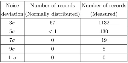
In Table 1, we show the number of records that should deviate more than 3, 5, 7, 9 and 11σ assuming a normal distribution, and the actual number of records from our 50,000 data points sample that do deviate.

1000 2000 3000 4000 5000

Record number -20

0 20 40

Temperature (Degrees C)

1000 2000 3000 4000 5000

Record number -4

-2 0 2 4 6

Difference (Degrees C)

Fig. 4.Plot of the temperature recorded from the two temperature sensors (top) and the difference (residuals) between the two readings (bottom).

Table 1.Analysed results from 50,000 readings.

Noise Number of records Number of records

deviation (Normally distributed) (Measured)

3σ 67 1132

5σ <1 130

7σ 0 19

9σ 0 8

11σ 0 0

investigation revealed that this effect was caused by the physical location of the two temperature sensors. One of the sensors is on the east side of the node, and the other on the west side of the node. As the sun rises in the morning, the east sensor warms more quickly than the west sensor causing a large (∼2 degree) temperature differential. However, during the course of the day, this difference reduces and becomes unnoticeable. However, as this is a regular, systematic effect, it does not change our methodology for detecting sensor faults.

3.2 Solar radiation sensor.

In order to do self-diagnosis on the solar radiation sensor, we have adopted a different approach to that used for the temperature sensors. As we only have one solar radiation sensor, we cannot use the same statistical method described above.

However, we do have access to the output voltage measured where the solar panel connects to the battery and this give us a direct reading of the output voltage of the solar panel (plus the battery voltage). Therefore, we should see a strong correlation between the voltage from the solar radiation sensor and the solar panel voltage.

Figure 5 shows the correlation for a period of three days, and Figure 6 shows the solar radiation sensor output voltage plotted against the solar panel voltage for 72,000 readings. As can be seen, there is a clear envelope that all the data lie within, showing a strong correlation between the two readings.

The observed hysterisis type appearance is due to the charging cycle of the battery. In the early morning (before dawn), the battery level is low (typically

∼13 volts) and during the course of the day the battery charges up, so that after dusk its voltage level is∼14 volts. The battery then discharges back to 13 volts during the course of the night, and the cycle repeats.

3.50•104 _3.60•104 _3.70•104 _3.80•104 _3.90•104 _4.00•104

Record number 0

200 400 600 800 1000 1200

Solar radiation (Watts per square metre)

3.50•104

3.60•104

3.70•104

3.80•104

3.90•104

4.00•104

Record number 12

13 14 15 16 17

Battery + Solar panel voltage (V)

Fig. 5. Three days of data illustrating the correlation between the solar radiation intensity, and the measured solar panel + battery voltage.

12 13 14 15 16 17

Battery + Solar panel voltage (V) 0

200 400 600 800 1000

Soalr radiation (Watts per square metre)

Fig. 6.Correlation between solar radiation intensity and solar panel + battery output voltage for 72,000 records.

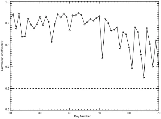
r=

P

i(xi−x)(yi−y) pP

i(xi−x)2pPi(yi−y)2

where (xi, yi), i= 1, . . . , N represent the measured values of the battery + solar panel voltage and the solar radiation sensor respectively, andxis the mean ofx andy is the mean ofy [18].

20 30 40 50 60 70

Day Number 0.5

0.6 0.7 0.8 0.9 1.0

Correlation coefficient r

Fig. 7.Correlation coefficient,r, plotted for a 50 day period.

By using Equation 1, we calculated the daily correlation coefficient, r, be-tween solar radiation and battery level for a 24 hour period. Figure 7 is a the plot of r for fifty days for the data set shown in Figure 6. These data illus-trate that the daily correlation coefficient between solar radiation and battery + solar panel voltage is always greater than 0.6, even on very overcast days. Therefore, based on this analysis, we set a threshold value, rth, of 0.6 in our

self-diagnostic algorithm. A calculated value of r < rth will flag an alert of a

possible degradation in the performance of either the solar panel, or the solar radiation sensor.

3.3 Anemometer diagnosis.

This established the following rule.

IF (Wdis changing) and (Wsis unchanged for 30 mins)

THEN ReportFault (2)

and

IF (Ws >2 mph) and (Wdis unchanged for 30 mins)

THEN ReportFault (3)

whereWdis the measured wind direction andWsis the measured wind speed.

3.4 Algorithm testing.

In order to test out self-diagnosis routines we forced a failure condition upon several of the sensors to ascertain the robustness of the self-diagnosis routines, and their ability to generate the appropriate alarm event.

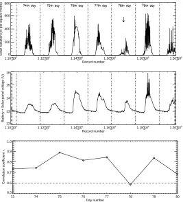
In one test, the solar radiation sensor was totally obscured for a period of one hour. Figure 8 (top plot) shows the point (indicated arrow) where the sensor was covered, at approximately noon, on the 78th

day, and the middle graph shows the corresponding solar panel voltage.

The bottom plot of Figure 8 shows the correlation coefficient, r, between the two datasets. Each point is the correlation coefficient as calculated from the previous 24 hours of data. Also shown is our phenomenologically determined threshold value ofrth= 0.6. As can be seen, the value ofrdrops belowrth and

an alarm signal was generated.

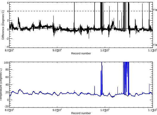
3.5 Detection of a real sensor failure.

During the latter part of the tests conducted above, we frequently received alerts indicating a failure of one of the temperature sensors. In Figure 9 (top), we have plotted the residuals for the two temperature sensors over the period in question, and our 11σ threshold level. As can be seen, there are many points where the data exceeded this threshold. The bottom graph of Figure 8 shows the raw data for the sensor. Clearly one of the sensors is faulty as it is intermittently recording temperatures in excess of 100o

centigrade!

1.10•105 _1.12•105 _1.14•105 _1.16•105 _1.18•105 _1.20•105

Record number 0

200 400 600 800

Solar radiation (W per square metre)

1.10•105 _1.12•105 _1.14•105 _1.16•105 _1.18•105 _1.20•105

Record number 12

13 14 15 16

Battery + Solar panel voltage (V)

73 74 75 76 77 78 79 80

Day number 0.5

0.6 0.7 0.8 0.9 1.0

Correlation coefficient r

Fig. 8.Solar radiation and solar panel + battery voltage, indicating a forced failure of the solar radiation and detection of the failure.

3.6 Towards self-adaptability.

In the proceeding analysis and examples, our node reacted solely on a fixed set of conditions imposed upon it; ie., ”if X>Y generate event”. However, we have anticipated the need for these set of conditions to be modifiable, either by the management system or the node itself, as the base-line performance of the node changes during its deployment. As a simple example, we consider the possible long term degradation of the solar radiation sensor caused by buildup of deposits on the transparent external casing of the sensor. This would manifest itself as a weakening of the correlation between its output and that of the solar panel. In order to compensate for any such degradation, the node can actively update the value ofrth required to generate an alert by performing a running average over

8.0•104 _9.0•104 _1.0•105 _1.1•105

Record number -4

-2 0 2 4 6

Difference (Degrees C)

8.0•104 _9.0•104 _1.0•105 _1.1•105

Record number -20

0 20 40 60 80 100

Temperature (Degrees C)

Fig. 9.Detecting a real failure of one of the temperature sensors.

4

Conclusions and further work.

Previous approaches to self-diagnostics routines have involved WSNs with ac-cess to powerful CPUs, a high level of human supervision, short (in the field) deployment times and/or a large data transmission requirement

We have identified the need for a WSN self-diagnostic routine that can be implemented autonomously on a low power microprocessor for periods in excess of a year.

By using readily available off-the-shelf components we have constructed a prototype sensor node that can be quickly deployed. Using the data from this deployed node, we have successfully developed and trialled a light weight, robust, rule-based self-diagnostic algorithm that very sucessfully detects sensor faults. Since its deployment in July 2006, the algorithm has sucessfully reported the failure of one of the temperature sensors, and (just as importantly)notgenerated any false-positive alarm events.

Our experimental results shows that this approach has a low computing com-plexity and achieves a high probability of correct diagnosis. It can be imple-mented on a broad set of low power microprocessors that have limited memory and processing speed.

Acknowledgments

The authors would like to thank EPSRC (Engineering and Physical Sciences Research Council) for funding this project and the mechanical workshop of the Electronics Department of the University of Kent for their invaluable technical assistance.

Addendum

Since this work was initially carried out and submitted, the authors, with the exception of Dr. Jonathan Stott, have relocated to Infolab21, Department of Computing, University of Lancaster, Lancaster, UK, LA1 4WA.

References

1. PROSEN. (2007) Prosen project homepage. [Online]. Available:

http://www.prosen.org.uk

2. P. Caselitz, J. Giebhardt, and M. Mevenkamp, “Application of condition

moni-toring systems in wind energy converters,” inEuropean Wind Energy Conference

(EWEC’97), Dublin, October 1997.

3. C. Angeli and A. Chatzinikolaou, “On-line fault detection techniques for technical

system: A survey,” International Journal of Computer Science & Applications,

vol. I, no. 1, pp. 12–30, 2004.

4. S. I. Roumeliotis, G. S. Sukhatme, and G. A. Bekey, “Sensor fault detection

and identification in a mobile robot,” in1998 IEEE International Conference on

Robotics and Automation, May 1998, pp. 2223–2228.

5. N. de Freitas, R. Dearden, F. Hutter, R. Morales-Menendez, J. Mutch, and

D. Poole, “Diagnosis by a waiter and a mars explorer,”Proceedings of IEEE, vol. 92,

no. 3, pp. 455–468, 2004.

6. P. Goel, G. Dedeoglu, S. I. Roumeliotis, and G. S. Sukhatme, “Fault detection and identification in a mobile robot using multiple model estimation and neural

network,” inIEEE International Conference on Robotics and Automation, Leuven,

Belgium, May 1998.

7. N. Ramanathan, L. Balzano, M. Burt, D. Estrin, T. Harmon, C. Harvey, J. Jay, E. Kohler, S. Rothenberg, and M. Srivastava, “Rapid deployment with confidence: Calibration and fault detection in environmental sensor networks,” Center for Em-bedded Networked Sensing, UCLA and Department of Civil and Environmental Engineering, MIT, Tech. Rep. CENS Tech Report 62, April 2006.

8. F. Koushanfar, M. Potkonjak, and A. Sangiovanni-Vincentelli, “On-line fault

de-tection of sensor measurements,” inSensors, 2003. Proceedings of IEEE, October

2003, pp. 974–979.

9. J. Bertrand-Krajewski, J. Bardin, M. Mourad, and Y. Beranger, “Accounting for sensor calibration, data validation, measurement and sampling uncertainities in

monitoring urban drainage systems.”Water Science and Technology, vol. 47, no. 2,

pp. 95–102, 2003.

10. J. Chen, S. Kher, and A. Somani, “Distributed fault detection of wireless sensor

networks,” in DIWANS ’06: Proceedings of the 2006 workshop on Dependability

11. (2006) Davis instruments, wireless vantage pro2 specifications. [Online]. Available: http://www.davisnet.com/support/weather/

12. CR200 Series Datalogger with Spread Spectrum Radio, Campbell Scientific, Inc., 2005.

13. RF401/RF411/RF416 Spread Spectrum Data Radio/Modem, Campbell Scientific, Inc., 2005.

14. H. Liet al., In prep., 2007.

15. J. Stott. (2006) Canterbury weather website. [Online]. Available:

http://www.canterburyweather.co.uk/

16. (2007) Uk weather extremes. [Online]. Available:

http://www.metoffice.gov.uk/climate/uk/extremes/index.html

17. Model 109 Temperature Probe User guide. Campbell Scientific Inc., 2002.

18. W. H. Press, S. A. Teukolsky, W. T. Vetterling, and B. P. Flannery, Numerical

recipes in C. New York, USA: Cambridge university press, 1992.