Performance comparison of path planning methods

(1)

www.arpnjournals.com

PERFORMANCE COMPARISON OF PATH PLANNING METHODS

Omar R. B., Che Ku Melor C. K. N. A. H. and

Sabudin E. N.

Faculty of Electrical and Electronic Engineering, Universiti Tun Hussein Onn Malaysia (UTHM), 86400 Parit Raja, Batu Pahat, Johor, Malaysia

E-Mail: roslio@uthm.edu.my

ABSTRACT

Path planning is one of the most vital aspects in robotics. Since the last few decades, it importance has been increasing due to the growing effort on the development of autonomous robots. Cell decomposition (CD), voronoi diagram (VD), probability roadmap (PRM) and visibility graph (VG) are among the earliest, most established and most popular methods in path planning. They have been used in many robotics path planning applications especially for autonomous systems. Before designing a path planning method, the three criteria i.e, path length, computational complexity and completeness have to be taken into account. This paper compares the performance of the above-mentioned path planning methods in terms of computation time and path length. For the sake of fair and conclusive finding, simulation is performed in three type of environments i.e., slightly cluttered, normally cluttered and highly cluttered. The finding shows that the visibility graph consistently produces relatively the shortest path while the voronoi diagram the longest. Shortest path is favorable for robots as the robots will consume less power/fuel and have an increased life cycle. However, the visibility graph is computationally intractable as in runs in polynomial time with respect to the number of obstacles. In contrast, PRM consumes the least time in planning a collision-free path. The finding of this paper could be used as a guideline about the performance in terms of path length and computation time for those who are interested in path planning using these four methods.

Key words: path planning, cell decomposition, voronoi diagram, probability roadmap (PRM), visibility graph

INTRODUCTION

From a technical perspective, path planning is a problem of determining a path for a robot in a properly defined environment from an initial point pinit to an end point pend

such that the robot is free from collisions with surrounding obstacles and its planned motion satisfies the robot’s physical/kinematic constraints (Hasircioglu et al., 2008) Typically, path planning of a robot A consists of two phases. The first phase is called the pre-processing phase in which nodes and edges (lines) are built within an environment/workspace W with A and obstacles O. In this phase, it is common to apply the concept of a configuration space (C-space) to represent A and O in W (Lozano- Perez, 1979), (Giesbrecht, 2004). In C-space, the robot’s size is reduced to a point, and the obstacles’ sizes are enlarged according to the size of A. Next, representation techniques are used to generate maps of graphs. Each technique differs in the way the nodes and edges are defined.

The second phase is termed the query phase in which a search for a path from pinit to pend is performed using (graph)

search algorithms. In this paper, Dijkstra’s algorithm is applied as it guarantees that the planned path is the shortest. Dijkstra’s algorithm measures the distance of a node n (g(n)) with respect to the pend. The cost at the node is

non-negative and has the cost of

𝑓(𝑛) = 𝑔(𝑛)

f(n) is also called the backward cost or cost-to-come. As the cost is non-negative, it is monotonically increased.

Path planning is closely related to autonomy as it may increase the capability of a robot to make its own decision based on the information presently available captured by

sensors, and potentially covers the whole range of the vehicle’s operations with minimal human intervention (Frampton, 2008). Autonomy increases system efficiency because all decisions are executed onboard except for critical decisions that have to be made by humans (Mitch et al., 2007).

Additionally, as introduced in (Eric, 2007), there are ten autonomy levels (applied to Unmanned Aerial Vehicle (UAV)) known as Autonomous Control Level (ACL). The concept of ACL as a metric to describe the autonomy in UAVs is widely accepted. Readers are referred to (Eric, 2007) for a detailed description of ACL. The most recent effort to address the issue of autonomy of UAVs is done by (Tanzi et al., 2014).

Path planning related problems have been extensively investigated and solved by many researchers (Nilsson, 1969), (Tokuta, 1998), (Yu et al., 2015). The important criteria for path planning that are commonly taken into account are computational time, path length and completeness. A path planning algorithm with less computational time is vital in real time application, which is desirable in dynamic environments. The generated optimal path in terms of path length by a path planning technique will minimise the mission time and hence prolongs the robot’s endurance and life cycle, minimises fuel/energy consumption and reduces exposure to possible risks. On the other hand, if a path planning method could find a path (if the path exists), it means that the method satisfies the completeness criterion.

(2)

0 100 200 300 400 500 600 700 800 0 100 200 300 400 500 600 700 800 1 2 3 4 5 6 7 8 9 10 11 12 13 14 15 16 17 18

19 21 20

22 23 24 25 26 27 28 29 30 31 32 33 34 35 36 37 38 39 40 41 42 43 44 45 46 47 48 49 50 x[unit] y [u n it ]

Path planning using Cell Decomposition in 750 x 750 units search space

0 100 200 300 400 500 600 700 800

0 100 200 300 400 500 600 700 800 x[unit] y [u n it ]

Path planning using Probabilistic Roadmap in 750 x 750 units search space

0 100 200 300 400 500 600 700 800

0 100 200 300 400 500 600 700 800 1 2 3 4 5 6 7 8 9 10 11 12 13 14 15 16 17 18

19 21 20

22 23 24 25 26 27 28 29 30 31 32 33 34 35 36 37 38 39 40 41 42 43 44 45 46 47 48 49 50 1 2 3 4 5 6 7 8 9 10 11 12 13 14 15 16 17 18

19 21 20

22 23 24 25 26 27 28 29 30 31 32 33 34 35 36 37 38 39 40 41 42 43 44 45 46 47 48 49 50 x[unit] y [u n it ]

Path planning using Voronoi Diagram in 750 x 750 units search space an optimal path is required. In this paper, the performance

of the cell decomposition (CD), voronoi diagram (VD), probability roadmap (PRM) and visibility graph (VG) will be investigated and compared with each other. The result may be useful for those who are looking for those methods for path planning.

ASSUMPTIONS

This paper considers path planning problem for a robot in a two-dimensional (2D or ℝ2_{) environment through} stationary polygonal obstacles, 𝑂 = {𝑂1, … , 𝑂𝑛} ⊂ ℝ2, from a designated initial point pinit to the end point pend using CD,

VD, PRM and VG methods. It is assumed that the environments are well-built urban areas and 𝑂 are hard, rectangle-shaped obstacles (buildings). It is also assumed that the knowledge of the entire environment such as the geometries, dimensions and locations of 𝑂 are known a-priori either from surveillance, satellite data or other means. The resultant path has to be collision-free.

[image:2.595.323.517.177.340.2]

OVERVIEW OF PATH PLANNING METHODS CD are among the most popular methods to represent the environment especially for outdoor scenarios as it is the most straightforward technique (Zhu et al., 1995), (Dudek et al., 2000). This is due to the fact that the cells can represent anything such as free space or obstacles (Giesbrecht, 2004). The first step in CD is to divide the C-space into simple, connected regions termed cells (Russell et. al., 2003). The cells are regions that might be square, rectangular or polygonal in shape. They are discrete, non-overlapping but adjacent to each other. If the cell contains obstacle (or part of obstacle), it is marked as occupied, otherwise it is marked as obstacle free. A connectivity graph is then constructed and a graph search algorithm is used to find a path throughout the cells from the initial point to the end point. In order to increase the quality of the path, the size of the cells has to be made smaller, which in turn increases the grid’s resolution, and hence computational time. An example of path planning using CD is shown in Figure 1.

Figure 1: Path planning using CD.

Note that the obstacles (black rectangles) and the regions shaded by black lines are the occupied ones while the region shaded by yellow lines are obstacle-free. The red, linear piece-wise segments are the resulting path.

Many researches have used VD for path planning (Xiao et al., 2006), (Bhattacharya et al., 2007), ( Shao et.

[image:2.595.55.248.541.697.2]

al., 2010). VD defines nodes as points that are equidistant from all the points’ surrounding obstacles. The paths generated from a graph by VD are relatively highly safe due to the fact that the edges of the paths are positioned as far as possible from the obstacles. However, the paths are inefficient and not optimal in terms of path length. Figure 2 shows an example of path planning using VD. The dashed black lines are the resulting path.

Figure 2: Path planning using VD.

On the other hand, PRM is a popular method for path planning as it is easy to apply (Kavraki et al., 1996), (Song et al., 2003), (Belghith et al., 2006). It is a learning approach, attempts to make planning in large or high-dimensional spaces tractable. It provides a good approximation of the connectivity of the configuration space area. This method consists of two phases i.e. learning phase and query phase. Learning phase constructs and stores the PRM. Learning phase constructs a graph G whose nodes are on the free area and edges connect the nodes without intersecting any obstacle. On the other hand, query phase connects pinit and pend to G. A search algorithm is then used

to find a path from pinit to pend. Figure 3 shows an example

of PRM used in path planning, in which the dashed cyan lines form a connectivity graph that connect sample points to their nearby neighbours points while the resulting path is represented by the dashed green lines.

Figure 3: Path planning using PRM.

[image:2.595.324.515.567.732.2]

(3)

0 100 200 300 400 500 600 700 800 0

100 200 300 400 500 600 700 800

x[unit]

y

[u

n

it

]

Path planning using Visibility Graph in 750 x 750 units search space

0 100 200 300 400 500 600 700 800

x[unit]

y

[u

n

it

]

Path planning using Probabilistic Roadmap in 750 x 750 units search space

0 100 200 300 400 500 600 700 800 0

100 200 300 400 500 600 700 800

x[unit]

y

[u

n

it

]

0 100 200 300 400 500 600 700 800 0

100 200 300 400 500 600 700 800

x[unit]

y

[u

n

it

]

0 100 200 300 400 500 600 700 800 0

100 200 300 400 500 600 700 800

x[unit]

y

[u

n

it

]

[image:3.595.71.264.103.265.2]

lines. The length for the normal PRM path is 1042.9 units while the pruned one is 1036.8.

Figure 4: Path planning using PRM with pruning.

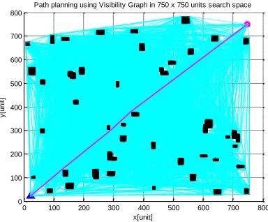
[image:3.595.330.513.334.509.2]

On the other hand, VG uses the vertices of the obstacles including the starting and target points in the C-space as the nodes. A VG network is then formed by connecting pairs of mutually-visible nodes by a set of edges E. A pair of mutually-visible nodes means that those nodes can be linked by a line/edge 𝑒 ∈ 𝐸 that does not intersect with any edge of obstacles in the C-space. Additionally, there is a cost associated with each E, possibly in terms of Euclidean distance. VG has been used by many researchers for path planning purpose including (Oommen et al., 1987), (Rao, 1989), (Tokuta, 1998). Figure 5 shows the path planned by VG in a random scenario. Note that the edges are represented by the cyan lines while the resulting path is in magenta.

Figure 5: Path planning using VG.

SIMULATION SETUP

Simulation was performed in scenarios, in which the number of obstacles were set to 25 (less-cluttered), 50 (normally-cluttered) and 75 (highly-cluttered). Example of these scenarios are illustrated in Figures 6(a) – 6(c). Note that the blue triangle is pinit while the magenta square is

pend.

To get a fair and conclusive result, for each method, 100 simulations were performed using 100 random scenarios for each number of obstacles. A desktop computer equipped

with an Intel i5 3360M, 2.40 GHz processor and 2GB RAM was used for such purpose.

Figure 6(a): A random scenario with 25 obstacles.

Figure 6(b): A random scenario with 50 obstacles.

[image:3.595.59.251.481.640.2] [image:3.595.328.511.551.728.2]

(4)

0 20 40 60 80 100 0

0.5 1 1.5 2 2.5

Simulation number

C

o

m

p

u

ta

ti

o

n

t

im

e

(s

e

c

o

n

d

)

Computation time with 25 obstacles

CD PRM PRM-pruned VD VG

0 20 40 60 80 100

0 0.5 1 1.5 2 2.5

Simulation number

C

o

m

p

u

ta

ti

o

n

t

im

e

(s

e

c

o

n

d

)

0 20 40 60 80 100

0 1 2 3 4 5 6

Simulation number

C

o

m

p

u

ta

ti

o

n

t

im

e

(s

e

c

o

n

d

)

RESULTS AND DISCUSSION

The simulation result in terms of computation time for 100 random scenarios with 25 obstacles is shown in Figure 7. The minimum, average and maximum computation time for each method is shown in Table 1. It is concluded that, from the table, PRM methods had the shortest computation time with an average of 0.07 seconds and a maximum of 0.12. On the other hand, CD had the highest average and maximum computation time, i.e. 1.89 and 2.37 seconds, respectively. This is due to the fact that creating the cell consumed a considerable time which leads to the higher computation time. Table 1 also shows that VD had a faster average computation time, i.e 0.14 seconds compared to VG, which used 0.41 seconds in average.

Figure 7: Computation time in environment with 25 obstacles.

Table 1: Computation time in environments with 25 obstacles.

Computation time (s)

Method Min Ave Max

CD 1.77 1.89 2.37

PRM 0.07 0.07 0.12

PRM-Pruned 0.07 0.07 0.13

VD 0.10 0.14 0.26

VG 0.35 0.41 0.57

As the number of obstacles increased to 50, the computation time of VD and VG in finding collision-free paths were also increased as illustrated by Figure 8. Table 2 lists the minimum, average and maximum time for each method in 100 random scenarios with 50 obstacles.

From Table 2, it is found that the average computation time of VD and VG were 0.62 and 1.87 seconds, respectively. This shows that the increment in the obstacles number has significantly increased the computation time of VD and VG. However, the simulation with 50 obstacles shows that the computation time of CD and both PRM methods have increased slightly as compared to the one with 25 obstacles.. With a further increment of obstacles number to 75, the computation time of each method in highly-cluttered environment is as depicted by Figure 9. The minimum,

average and maximum computation time for each method in 100 scenarios with 75 obstacles is listed in Table 3, which shows that the computation time of VG is significantly increased to an average of 4.50 seconds.

The average computation time of VD is also increased to 1.59 seconds, but not as abrupt as that of VG. It is also observed that both PRMs had a slight increase in the computation time when the obstacles number was raised from 50 to 75. However, the computation time of CD is almost identical with those in the scenarios with 50 obstacles.

Figure 8: Computation time in environment with 50 obstacles.

CD 1.73 1.87 2.39

PRM 0.15 0.17 0.25

PRM-Pruned 0.15 0.17 0.25

VD 0.40 0.62 1.24

VG 1.58 1.87 2.35

[image:4.595.318.536.218.394.2] [image:4.595.61.283.251.432.2] [image:4.595.314.549.479.753.2] [image:4.595.49.288.525.610.2]

(5)

0 20 40 60 80 100 1100

1200 1300 1400 1500 1600 1700

Simulation number

P

a

th

l

e

n

g

th

[u

n

it

]

Paths lengths with 25 obstacles

0 20 40 60 80 100

1100 1200 1300 1400 1500 1600 1700

Simulation number

P

a

th

l

e

n

g

th

[u

n

it

]

0 20 40 60 80 100

1100 1200 1300 1400 1500 1600 1700

Simulation number

P

a

th

l

e

n

g

th

[u

n

it

]

CD 1.73 1.87 2.39

PRM 0.27 0.30 0.40

PRM-Pruned 0.27 0.30 0.41

VD 0.90 1.59 4.53

VG 3.91 4.50 5.25

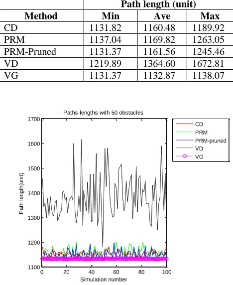
As for the path length, it is found that VG produced the shortest path among the methods as illustrated in Figures 10 to 12. This is due to the fact that the waypoints of VG’s path pass through the nodes of certain obstacles. As listed in Tables 4 to 6, it is observed that the average path length for each method did not change significantly with the increase of obstacles numbers.

Comparing the average path lengths of PRM and PRM-pruned from Tables 4 to 6, it is found that the latter produced a slightly shorter path although consumed a bit longer computation time than the former. This advantage, although small, is particularly useful for a robot in saving its energy/fuel and having a longer life cycle.

[image:5.595.48.288.111.196.2]

Figure 10: Path length in environment with 25 obstacles.

Table 4: Lengths of the planned path in environments with 25 obstacles.

Path length (unit)

CD 1131.82 1142.28 1170.55

PRM 1132.07 1152.35 1214.01

PRM-Pruned 1131.37 1142.71 1205.76

VD 1145.25 1374.53 1666.17

VG 1131.37 1131.70 1132.79

Table 5: Lengths of the planned paths in environments with 50 obstacles.

CD 1131.82 1153.41 1180.24

PRM 1136.66 1160.77 1201.46

PRM-Pruned 1131.37 1150.11 1194.78

VD 1181.10 1382.62 1615.57

[image:5.595.315.549.256.542.2]

VG 1131.37 1132.30 1134.66

Table 6: Lengths of the planned paths in environments with 75 obstacles.

CD 1131.82 1160.48 1189.92

PRM 1137.04 1169.82 1263.05

PRM-Pruned 1131.37 1161.56 1245.46

VD 1219.89 1364.60 1672.81

[image:5.595.57.274.400.576.2]

VG 1131.37 1132.87 1138.07

Figure 11: Path length in environment with 50 obstacles.

[image:5.595.329.551.575.755.2]

(6)

CONCLUSION

The paper has demonstrated the performance of a number of established and popular methods used in path planning i.e.,

cell decomposition (CD), voronoi diagram (VD),

probabilistic roadmaps (PRMs) and visibility graph (VG). It was found that VG produced shortest path consistently. However, the computation time of VG was exponentially increased with respect to the number of obstacles. With the above-mentioned advantage, it is worth researching on VG to improve its computation time. On the other hand, VD had a consistent increment in computation time as the number of obstacles was increased. As for CD and both PRMs, the computation time were almost identical in slightly-, normally- and highly-cluttered environments. All four methods showed a minimal increase in path length as the number of obstacles increased.

ACKNOWLEDGEMENT

This work is supported by Universiti Tun Hussein Onn Malaysia (UTHM) and funded by Vot 1489 of Fundamental Research Grant Scheme (FRGS).

REFERENCE

Hasircioglu, I., Topcuoglu, H. R. and Ermis, M. (2008). 3-D path planning for the navigation of unmanned aerial vehicles by using evolutionary algorithms. Proceedings of the Conference on Genetic and Evolutionary Computation, pp. 1499--1506.

Giesbrecht, J. (2004). Path planning for unmanned ground vehicles. Technical Memorandum DRDC Suffield TM 2004-272.

Frampton, R. (2008). UAV autonomy, In MOD Codex

Journal, Issue 1 Summer, 2008, [Online]

www.science.mod.uk/codex/Issue1/Journals/documents/Iss ue1_2Journals_UAV_auto nomy.pdf .

Mitch, F., Tu, Z., Stephens, L. and Prickett, G. (2007). Towards true UAV autonomy. Proceedings of the IEEE International Conference on Information, Decision and Control, pp. 170-175, 2007.

Eric, S. (2007). Evolution of a UAV autonomy classification taxonomy. Proceedings of the IEEE International Conference on Aerospace.

Nilsson, N.J. (1969). A mobile automaton: An application of artificial intelligence techniques. Proceedings of International Joint Conference on Artificial Intelligence, pp. 509--520.

Tokuta, A. (1998). Extending the VGRAPH algorithm for robot path planning. In International Conference in Central Europe on Computer Graphics and Visualization.

Zhu, D. and Latombe, J. (1995). Constraint reformulation in hierarchical path planning. Proceedings of the IEEE/RSJ International Conference on Intelligent Robots and Systems, pp. 1918--1923.

Dudek, G. and Jenkin, M. (2000). Computational principles of mobile robotics. Cambridge University Press, Cambridge, UK.

Russell, S. J. and Norvig, P. (2003). Artificial intelligence: A modern approach, 2nd_{Edition, Prentice Hall, Upper}

Saddle River, N.J.

Xiao, Q., Gao, X., Fu, X. and Wang, H. (2006). New local path re-planning algorithm for unmanned combat air vehicle. Proceedings of the 6th World Congress on Intelligent Control and Automation, pp. 4033--4037.

Shao, M and Lee, J. Y. (2010). Development of autonomous navigation method for non-holonomic mobile robots based on the generalized voronoi diagram. Proceedings of the IEEE International Conference on Control Automation and Systems, pp. 309--313.

Bhattacharya, P. and Gavilova, M. L. (2007). Voronoi diagram in optimal path planning. Proceedings of the IEEE International Symposium on Voronoi Diagrams in Science and Engineering, pp. 38--47.

Kavraki, L.E., Svestka, P., Latombe, J.-C. and Overmars, M.H. (1996). Probabilistic roadmaps for path planning in high-dimensional configuration spaces. Robotics and Automation, IEEE Transactions on , vol.12, no.4, pp.566— 580.

Song, G., Thomas, S. and Amato, N. M. (2003). A General Framework for PRM Motion Planning. Proceedings of the 2003 IEEE International Conference on Robotics &Automation pp. 4445--4450.

Belghith, K., Kabanza, F., Hartman, L. and Nkambou, R. (2006). Anytime Dynamic Path-Planning with Flexible Probabilistic Roadmaps. Proceedings of the 2006 IEEE International Conference on Robotics and Automation, pp. 2372--2377.

Oommen, B. J., Iyengar, S., Rao, N. S. V. and Kashyap, R. L.(1987). Robot navigation in unknown terrains using learned visibility graphs. Part I: The disjoint convex obstacle case. IEEE Journal of Robotics and Automation, RA-3(6), pp. 672--681.

Rao, N. S. V. (1989). Algorithmic framework for learned robot navigation in unknown terrains. Journal of Computer, 22(6), pp 37--43.

Tanzi, T., Apvrille, L., Dugelay, J.-L. and Roudier, Y. (2014) UAVs for humanitarian missions: Autonomy and reliability, Global Humanitarian Technology Conference (GHTC), 2014 IEEE, pp.271--278.

Yu, H., Meier, K., Argyle, M. and Beard, R.W. (2015). Cooperative Path Planning for Target Tracking in Urban

Environments Using Unmanned Air and Ground