R E S E A R C H
Open Access
Adaptively relaxed algorithms for solving the
split feasibility problem with a new step size
Haiyun Zhou
1,2and Peiyuan Wang
2,3*Dedicated to Professor Shih-sen Chang on his 80th birthday
*Correspondence:
2Department of Mathematics,
Shijiazhuang Mechanical Engineering College, Shijiazhuang, 050003, China
3The Second Training Base, Naval
Aviation Institution, Huludao, 125001, China
Full list of author information is available at the end of the article
Abstract
In the present paper, we propose several kinds of adaptively relaxed iterative algorithms with a new step size for solving the split feasibility problem in real Hilbert spaces. The proposed algorithms never terminate, while the known algorithms existing in the literature may terminate. Several weak and strong convergence theorems of the proposed algorithms have been established. Some numerical experiments are also included to illustrate the effectiveness of the proposed algorithms.
MSC: Primary 46E20; 47J20; secondary 47J25
Keywords: split feasibility problem; adaptive step size; adaptively relaxed iterative algorithm; convergence
1 Introduction
Since its inception in , the split feasibility problem SFP [] has been attracting searchers’ interest [, ] due to its extensive applications in signal processing and image re-construction [], with particular progress in intensity-modulated radiation therapy [, ]. LetHandHbe real Hilbert spaces,CandQbe nonempty closed convex subsets of
H andH, respectively, andA:H→H a bounded linear operator. Then SFP can be formulated as finding a pointxˆwith the property
ˆ
x∈C and Axˆ∈Q. (.)
The set of solutions for SFP (.) is denote by=C∩A–(Q).
Over the past two decades years or so, the researchers invested and designed various iterative algorithms for solving SFP (.); see [–]. The most popular algorithm, among them, is Byrne’s CQ algorithm, which generates a sequence{xn}by the recursive procedure
x∈H, xn+=PCxn–τnA∗(I–PQ)Axn, n≥, (.)
where the step sizeτnis chosen in the open interval (, /A), whilePCandPQare the
orthogonal projections ontoCandQ, respectively.
We remark in passing that Byrne’s CQ algorithm (.) is indeed a special case of the classical gradient projection method (GPM). To see this, let us definef :H→R by
f(x) =
(I–PQ)Ax
, (.)
then the convex objectivef is differentiable and has a Lipschitz gradient given by
∇f(x) =A∗(I–PQ)Ax. (.)
We consider the following convex minimization problem:
min
x∈Cf(x). (.)
It is well known thatxˆ∈Cis a solution of problem (.) if and only if
∇f(ˆx),x–xˆ≥, ∀x∈C. (.)
Also, we know that (.) holds true if and only if
ˆ
x=PC(I–τ∇f)ˆx, ∀τ> . (.)
Note that if=∅, thenxˆ∈⇔f(ˆx) =minx∈Cf(x)⇔(.) holds⇔(.) holds.
Conse-quently, we can utilize the classical gradient projection method (GPM) below to solve SFP (.):
x∈C, xn+=PC
xn–τn∇f(xn)
, n≥, (.)
whereτn∈(, /L), whileLis the Lipschitz constant of∇f. Noting thatL=A, we see
immediately that (.) is exactly CQ algorithm (.).
We note that, in algorithms (.) and (.) mentioned above, the choice of the step size τndepends heavily on the operator (matrix) normA. This means that for actual
im-plementation of CQ algorithm (.), one has first to know at least an upper bound of the operator (matrix) normA, which is in general difficult. To overcome this difficulty,
sev-eral authors proposed sevsev-eral various of adaptive methods, which permit the step sizeτn
to be selected self-adaptively; see [–]. Yang [] considered the following step size:
τn:=
ρn
∇f(xn)
, (.)
where{ρn}is a sequence of positive real numbers such that
∞
n=
ρn=∞,
∞
n=
ρn<∞. (.)
Very recently, Lópezet al.[] introduced another choice of the step size sequence{τn}
as follows:
τn:=
ρnfn(xn)
where{ρn}is chosen in the open interval (, ). By virtue of the step size (.), Lópezet al.[] introduced four kinds of algorithms for solving SFP (.).
We observe that if∇f(xn) = for somen≥, then the algorithms introduced by López et al.[] have to terminate in thenth step of iterations. In this casexnis not necessarily a solution of the SFP (.), sincexnmay be not inC, Algorithm . in [] is such a case. To make up the flaw, we introduce a new choice of the step size sequence{τn}as follows:
τn:=
ρnfn(xn) (∇fn(xn)+σn)
, (.)
where{ρn}is chosen in the open interval (, ) and{σn}is a sequence of positive numbers
in (, ), whilefnand∇fnare given by, respectively,
fn(x) =
(I–PQn)Ax
, (.)
∇fn(x) =A∗(I–PQn)Ax, (.)
where{Qn}will be defined in Section .
The purpose of this paper is to introduce a new choice of the step size sequence{τn}
that makes the associated algorithms never terminate. A new stop rule is also given, which ensures that the (n+ )th iterationxn+is a solution of SFP (.) and the iterative process stops. Several weak and strong convergence results are presented. Numerical experiments are included to illustrate the effectiveness of the proposed algorithms and the applications in signal processing of the CQ algorithm with the step size selected in this paper.
The rest of this paper is organized as follows. In the next section, some necessary con-cepts and important facts are collected. The weak and strong convergence theorems of the proposed algorithms with step size (.) are established in Section . Finally in Section , we provide some numerical experiments to illustrate the effectiveness and applications of the proposed algorithms with step size (.) to inverse problems arising from signal processing.
2 Preliminaries
Throughout this paper, we assume that SFP (.) is consistent,i.e.,=∅. We denote by Rthe set of real numbers. LetHandHreal Hilbert spaces and the letterIthe identity mapping onHorH. Iff :H→Ris a differentiable (subdifferentiable) functional, then we denote by∇f(∂f) the gradient (subdifferential) off. Given a sequence{xn}inH,ww(xn)
(resp. ‘xnx’) denotes the strong (resp. weak) convergence of{xn}tox. The symbols·,· and · denote inner product and norm of Hilbert spacesH andH, respectively. Let
T:H→Hbe a mapping. We useFix(T) to denote the set of fixed points ofT. We also denote bydom(T) the domain ofT.
Some equalities in Hilbert spaceHplay very important roles for solving linear and non-linear problems arising from real world.
It is well known that in a real Hilbert spaceH, the following two equalities hold:
for allx,y∈H.
tx+ ( –t)y=tx+ ( –t)y–t( –t)x–y, (.)
for allx,y∈Handt∈R.
Recall that a mappingT:dom(T)⊂H→His said to be
(i) nonexpansive if
Tx–Ty ≤ x–y, (.)
for allx,y∈dom(T); (ii) firmly nonexpansive if
Tx–Ty≤ x–y–(I–T)x– (I–T)y, (.)
for allx,y∈dom(T);
(iii) λ-averaged if there exist someλ∈(, )and another nonexpansive mapping S:H→Hsuch that
T= ( –λ)I+λS. (.)
The following proposition describes the characterizations of firmly nonexpansive map-pings (see []).
Proposition . Let T:dom(T)⊂H→Hbe a mapping.Then the following statements are equivalent.
(i) Tis firmly nonexpansive; (ii) I–Tis firmly nonexpansive;
(iii) Tx–Ty≤ x–y,Tx–Tyfor allx,y∈H; (iv) Tis
-averaged; (v) T–Iis nonexpansive.
Recall that the metric (nearest point) projection formHonto a nonempty closed convex
subsetCofHis defined as follows: for eachx∈H, there exists a unique pointPCx∈C
with the property:
x–PCx ≤ x–y, ∀y∈C. (.)
Now we list some basic properties ofPCbelow; see [] for details.
Proposition .
(p) Givenx∈Handz∈C.Thenz=PCxif and only if we have the inequality
(p)
PCx–PCy≤ x–y,PCx–PCy, for allx,y∈H; (.)
(p)
(I–PC)x– (I–PC)y≤(I–PC)x– (I–PC)y,x–y, (.)
for allx,y∈H.
(p) PC–Iis nonexpansive; (p)
PCx–PCy≤ x–y–(I–PC)x– (I–PC)y, x,y∈H; (.)
in particular, (p)
PCx–y≤ x–y–(I–PC)x, for allx∈Handy∈C. (.)
From (p), (p), and (p), we see immediately that bothPCand (I–PC) are firmly
non-expansive and-averaged.
Recall that a functionf :H→Ris called convex if
fλx+ ( –λ)y≤λf(x) + ( –λ)f(y), ∀λ∈(, ),∀x,y∈H.
It is well known that a differentiable functionfis convex if and only if we have the relation
f(z)≥f(x) +∇f(x),z–x, ∀z∈H.
Recall that an elementξ∈His said to be a subgradient off :H→Ratxif
f(z)≥f(x) +ξ,z–x, ∀z∈H.
If the functionf :H→Rhas at least one subgradient atx, it is said to be subdifferen-tiable atx. The set of subgradients off at the pointxis called the subdifferential off atx, and is denoted by∂f(x). A functionf is called subdifferentiable if it is subdifferentiable at everyx∈H. Iff is convex and differentiable, then∂f(x) ={∇f(x)}for everyx∈H. A functionf is called subdifferentiable if it is subdifferentiable at everyx∈H. Iff is con-vex and differentiable, then∂f(x) ={∇f(x)}for everyx∈H. A functionf:H→Ris said to be weakly lower semi-continuous (w-lsc) atxifxnximplies
f(x)≤lim n
f(xn).
f is said to be w-lsc onHif it is w-lsc at every pointx∈H.
It is well known that for a convex functionf :H→R, it is w-lsc onHif and only if it is lsc onH.
Proposition . Let f be given as in(.).Then the following conclusions hold.
(i) f is convex and differentiable; (ii) ∇f(x) =A∗(I–PQ)Ax,x∈H; (iii) f is w-lsc onH;
(iv) ∇f isA-Lipschitz:
∇f(x) –∇f(y)≤ Ax–y, x,y∈H.
The concept of Fejér monotonicity plays a key role in establishing weak convergence theorems. Recall that a sequence{xn}inHis said to be Fejér monotone with respect to (w.r.t.) a nonempty closed convex subsetCinHif
xn+–z ≤ xn–z, ∀n≥,∀z∈C.
Proposition .(see [, ]) Let C be a nonempty closed convex in H.If the sequence
{xn}is Fejér monotone w.r.t.C,then the following hold:
(i) xnxˆif and only ifww(xn)⊂C; (ii) the sequence{PCxn}converges strongly; (iii) ifxnxˆ∈C,thenxˆ=limnPCxn.
Proposition .(see []) Let{αn}be a sequence of nonnegative real numbers such that
αn+≤( –tn)αn+tnbn, n≥,
where{tn}is a sequence in(, )and bnis a sequence inRsuch that (i) ∞n=tn=∞;
(ii) limnbn≤or
∞
n=|tnbn|<∞.Thenαn→(n→ ∞).
3 Main results
Letc:H→Randq:H→Rbe convex functions and define level sets of candqas follows:
C= x∈H|c(x)≤ and Q= y∈H|q(y)≤. (.)
Assume that bothcandqare subdifferentiable onHandH, respectively, and that∂c
and∂qare bounded mappings. Given an arbitrary initial datax∈H. Assume thatxnis the current value forn≥. We introduce two sequences of half-spaces as follows:
Cn= x∈H|c(xn)≤ ξn,xn–x
, (.)
whereξn∈∂c(xn), and
Qn= y∈H|q(Axn)≤ ηn,Axn–y
, (.)
Constructxn+via the formula
xn+=PCn
xn–τn∇f(xn)
, (.)
where{τn}is given as (.),
fn(x) =
(I–PQn)Ax
(.)
and
∇fn(x) =A∗(I–PQn)Ax, (.)
More precisely, we introduce the following relaxed CQ algorithm in an adaptive way.
Algorithm . Choose an initial datax∈H arbitrarily. Assume that thenth iteratexn
has been constructed then we compute the (n+ )th iterationxn+via the formula:
xn+=PCn
xn–τn∇f(xn)
, n≥, (.)
where the step sizeτnis chosen in such a way that
τn:=
ρnfn(xn) (∇fn(xn)+σn)
, (.)
with <ρn< and <σn< . Ifxn+=xnfor somen≥, thenxn is a solution of the
SFP (.) and the iterative process stops; otherwise, we setn:=n+ and go on to (.) to compute the next iterationxn+.
We remark in passing that ifxn+=xnfor somen≥, thenxm=xnfor allm≥n+ , consequently,limm→∞xm=xnis a solution of SFP (.). Thus, we may assume that the
sequence{xn}generated by Algorithm . is infinite.
Theorem . Assume thatlimnρn( –ρn)≥ρ> .Then the sequence{xn}generated by Algorithm.converges weakly to a solutionx of SFPˆ (.),wherexˆ=limn→∞Pxn. Proof Letz∈be fixed, and setyn=xn–τn∇fn(xn). By virtue of (.), (.), and
Proposi-tion .(p), we have
xn+–z=PCnyn–z
≤ yn–z–yn–PCnyn
=xn–z–τn∇fn(xn)–yn–PCnyn
=xn–z– τn
∇fn(xn),xn–z–yn–PCnyn
+τn∇fn(xn)
In view of Proposition ., we know thatI–PQnare firmly nonexpansive for alln≥, and from this one derives
∇fn(xn),xn–z=(I–PQn)Axn,Axn–Az
=(I–PQn)Axn– (I–PQn)Az,Axn–Az
≥(I–PQn)Axn= fn(xn), (.)
from which it turns out that
xn+–z≤ xn–z– τnfn(xn) +τn∇fn(xn)–yn–PCnyn
=xn–z– ρnf
n(xn)
(∇fn(xn)+σn)
+ ρ
nfn(xn)
(∇fn(xn)+σn)
∇fn(xn)
–yn–PCnyn
≤ xn–z–ρn( –ρn) f
n(xn)
(∇fn(xn)+σn)
–yn–PCnyn
, (.)
which in turn allows us to deduce the following conclusions:
(i) {xn}is Fejér monotone w.r.t.; in particular, (ii) {xn}is a bounded sequence;
(iii) ∞n=ρn( –ρn)fn(xn)/(∇fn(xn)+σn)<∞; and (iv)
∞
n=
yn–PCnyn<∞. (.)
By Proposition .(i), to show thatxnx, it suffices to show thatww(xn)⊂. To see this, takex∗∈ww(xn) and let{xnk}be a sequence of{xn}weakly converging tox∗. By our assumption thatlimnρn( –ρn)≥ρ> , without loss of generality, we can assume that
ρn( –ρn)≥ρ for alln≥. It follows from (.) (iii) that
fn(xn) ∇fn(xn)+σn →
(n→ ∞). (.)
Note that∇fn(xn)+σn≤ Axn–z+ forz∈. This, together with (.),
im-plies thatfn(xn)→, that is,(I–PQn)Axn →. By our assumption that∂qis a bounded mapping, we see that there exists a constantM> such thatηn ≤M,∀ηn∈∂q(Axn).
SincePQn(Axn)∈Qn, by the definition ofQn, we have
q(Axn)≤ηn,Axn–PQn(Axn)
≤M(I–PQn)Axn→. (.)
Noting thatAxnk Axˆ and using the w-lsc ofq, we haveq(Ax∗)≤limkq(Axnk)≤, which implies thatAx∗∈Q. We next provex∗∈C. Firstly, from (.) (iv), we know that yn–PCnyn →. Notice that
yn–xn=τn∇fn(xn)≤
fn(xn) ∇fn(xn)+σn·
∇fn(xn) ∇fn(xn)+σn ≤
fn(xn) ∇fn(xn)+σn→
we have
xn–PCnxn ≤ xn–yn+yn–PCnyn+PCnyn–PCnxn
≤xn–yn+yn–PCnyn →.
Since∂cis a bounded mapping, we haveM> such that
ξ ≤M, ∀ξn∈∂c(xn).
SincePCn(xn)∈Cn, by the definition ofCn, we have
c(xn)≤ ξn,xn–PCnxn ≤M(I–PCn)xn→.
Then w-lsc ofCimplies thatc(x∗)≤limkc(xnk)≤, thusx∗∈Candww(xn)⊂,
complet-ing the proof.
We introduce a little more general algorithm as follows.
Algorithm . Choose an initial datax∈Harbitrarily. Assume that thenth iterationxn
has been constructed; then we compute the (n+ )th iterationxn+via the formula:
xn+=βnxn+ ( –βn)PCn
xn–τn∇f(xn)
, n≥, (.)
where the step size{τn}is as before and{βn}is a sequence in (, ) satisfyinglimnβn< .
Ifxn+=xnfor somen≥, thenxnis a solution of the SFP (.) and the iterative process stops; otherwise, we setn:=n+ and go on to (.) to compute the next iterationxn+.
We have the following weak convergence theorem.
Theorem . Assume thatlimnρn( –ρn)≥ρ> .Then the sequence{xn}generated by Algorithm.converges weakly to a solutionx of the SFPˆ (.)wherexˆ=limn→∞Pxn.
Proof Letz∈be fixed and setyn=xn–τn∇fn(xn). By virtue of (.), (.), (.), (.),
and Proposition .(p), we have
xn+–z=βn(xn–z) + ( –βn)(PCnyn–z)
=βnxn–z+ ( –βn)PCnyn–z–βn( –βn)xn–PCnyn
≤βnxn–z+ ( –βn)yn–z– ( –βn)yn–PCnyn
=βnxn–z+ ( –βn)xn–z–τn∇fn(xn)
– ( –βn)yn–PCnyn
=βnxn–z+ ( –βn)xn–z– ( –βn)τn
∇fn(xn),xn–z
+ ( –βn)τn∇fn(xn)
– ( –βn)yn–PCnyn
–βn( –βn)yn–PCnyn
≤ xn–z– ( –βn)ρn( –ρn)
fn(xn) (∇fn(xn)+σn)
– ( –βn)yn–PCnyn
, (.)
which implies that
(i) {xn}is Fejér monotone w.r.t.; in particular, (ii) {xn}is a bounded sequence;
(iii) ∞n=( –βn)ρn( –ρn)fn(xn)/(∇fn(xn)+σn)<∞; and (iv) ∞n=( –βn)yn–PCnyn<∞.
By our assumptions on{βn}and{ρn}, we have ∇fnfn(x(xnn))+σn→ andyn–PCnyn→, the rest of the arguments follow exactly form the corresponding parts of Theorem ., we
omit its details. This completes the proof.
We remark that Theorem . generalizes Theorem ., that is, if we takeβn≡ in
The-orem ., then we can obtain TheThe-orem .. It is really interesting work to compare con-vergence rate of Algorithms . and ..
Generally speaking, Algorithms . and . have only the weak convergence in the frame work of infinite-dimensional spaces, and therefore the modifications of Algorithms . and . are needed in order to realize the strong convergence. Considerable efforts have been made and several interesting results have been reported recently; see [–]. Below is our modification of Algorithms . and ..
Algorithm . Choose an arbitrary initial datax∈H. Assume that the nth iteration
xn∈Hhas been constructed. Set
yn=PCn
xn–τn∇f(xn)
, n≥, (.)
with the step sizeτngiven by (.), and define two half-spacesYnandZnby
Yn=
z∈H:yn–z≤ xn–z–ρn( –ρn) f
n(xn)
(∇fn(xn)+σn)
, (.)
Zn= z∈H:x–xn,z–xn ≤
. (.)
The (n+ )th iteratexn+is then constructed in the formula:
xn+=PYn∩Zn(x). (.)
Ifxn+=xnfor somen≥, thenxnis a solution of SFP (.) and the iterative process stops;
otherwise, we setn:=n+ and go on to (.)-(.) to compute the next iterationxn+.
Theorem . Assume thatlimnρn( –ρn)≥ρ> .Then the sequence{xn}generated by Algorithm.converges strongly to a solution x∗of SFP(.),where x∗=P(x).
Proof Firstly, we show that
for alln≥. Indeed, in view of (.), we have⊂Ynfor alln≥. To show (.) holds, it suffices to show that⊂Znfor alln≥. We complete the proof by induction. Since
Z=H,⊂Z. Assume that⊂Zk form somek≥; we plan to show⊂Zk+. Since ⊂Yk∩Zk, andYk∩Zk=∅closed convex,xn+=PYn∩Zn(x) is well defined. It follows
from Proposition .(p) that
xk+–z,xk+–x ≤, ∀z∈. (.)
This implies thatz∈Zk+and hence⊂Zk+. Consequently,⊂Znfor alln≥, and thus (.) holds true.
From the definition ofZnand Proposition .(p), we see thatxn=PZnx. It then follows from (.) that
xn–x=PZnx–x ≤ xn+–xn=PZn+x–x ≤ Px–x. (.)
This derives thatlimnxn–xexists, dented byd.
Noting thatxn+∈Zn, we have
xn+–xn,xn–x ≥. (.)
By virtue of (.) and (.), we obtain
xn+–x–xn–x=xn+–xn+ xn+–xn,xn–x ≥ xn+–xn. (.)
From this one derives thatxn+–xn→ (n→ ∞).
Sincexn+∈Yn, we have
yn–xn+≤ xn–xn+–ρn( –ρn) f
n(xn)
(∇fn(xn)+σn)
, (.)
from which it turns out that
yn–xn+ ≤ xn–xn+ → (.)
and
ρn( –ρn) f
n(xn)
(∇fn(xn)+σn)
≤ xn–xn+→. (.)
At this point, we showww(xn)⊂. To end this, takexˆ∈ww(xn). Then there exists a
sub-sequence{xnj}of{xn}such thatxnj
w
−→ ˆx. By our assumption thatlimnρn( –ρn)≥ρ> ,
from (.) we conclude that
fn(xn)
∇fn(xn)+σn →
, (.)
which implies thatfn(xn)→, since{∇fn(xn)+σn}is bounded. Notice thatPQn(Axn)∈
Qn, and∂qis a bounded mapping, we have
q(Axn)≤ηn,Axn–PQn(Axn)
SinceAxnjAxˆandqis w-lsc onH, we derive
q(Axˆ)≤lim j
q(Axnj)≤,
which implies thatAxˆ∈Q.
We next showxˆ∈C. Indeed, from (.) we have
yn–xn ≤ yn–xn++xn+–xn →. (.)
From (.), we have also
τn∇fn(xn)=
ρnfn(xn)
∇fn(xn)+σn·
∇fn(xn)
∇fn(xn)+σn≤
fn(xn)
∇fn(xn)+σn→
. (.)
Consequently, it follows from (.) and (.) that
xn–PCnxn ≤ xn–yn+yn–PCnxn
≤ xn–yn+τn∇fn(xn)→. (.)
SincePCn(xn)∈Cn, noting∂cis a bounded mapping, we immediately obtain
c(xn)≤ ξn,xn–PCnxn ≤M(I–PCn)xn→.
Then the w-lsc ofcensures that
c(ˆx)≤lim j
c(xnj)≤,
from which it turns out thatxˆ∈C, and thusxˆ∈. It follows from (.) thatxˆ∈Zn, which implies that
x–xn,xˆ–xn ≤, (.)
for alln≥. Thus, from (.) we obtain
xn–xˆ≤ ˆx–x,xˆ–xn, (.)
in particular, we have
xnj–xˆ
≤ ˆx–x
,xˆ–xnj,
consequently,xnj→ ˆx, sincexnj
w
−→ ˆx. At this point, by virtue of (.), we have
in particular, we have
x–xnj,z–xnj ≤, ∀z∈. (.)
Thus, upon taking the limit asj→ ∞in (.), we obtain
x–xˆ,z–xˆ ≤, ∀z∈. (.)
This implies that xˆ=Px by Proposition .(p). Therefore{xn} converges strongly to
ˆ
x=Pxbecause of the uniqueness ofPx. This completes the proof.
Algorithm . Choose an arbitrary initial datax∈H. Assume that the nth iteration
xn∈Hhas been constructed. Set
yn=βnxn+ ( –βn)PCn
xn–τn∇f(xn)
, (.)
with the step sizeτngiven by (.) and the relaxed factorβnin [, ) satisfyinglimnβn< .
Define two half-spacesYnandZnby
Yn=
z∈H:yn–z≤ xn–z–ρn( –ρn)
fn(xn) (∇fn(xn)+σn)
– ( –βn)xn–τn∇fn(xn) –PCn
xn–τn∇fn(xn)
, (.)
Zn= z∈H:x–xn,z–xn ≤. (.)
The (n+ )th iterationxn+is then constructed by the formula:
xn+=PYn∩Zn(x). (.)
Ifxn+=xnfor somen≥, thenxnis a solution of SFP (.) and the iterative process stops; otherwise, we setn:=n+ and go on to (.)-(.) to compute the next iterationxn+.
Along the proof lines of Theorem . we can prove the following.
Theorem . Assume thatlimnρn( –ρn)≥ρ> ;then the sequence{xn} generated by Algorithm.converges strongly to a solution x∗of SFP(.),where x∗=P(x).
The proof of Theorem . is similar to that of Theorem ., and therefore we omit its details.
We next turn our attention to another kind of algorithm.
Algorithm . Choose an arbitrary initial datax∈H. Assume that thenth iterationxn∈ Hhas been constructed; then we compute the (n+ )th iterationxn+via the recursion:
xn+=PCn
αng(xn) + ( –αn)
xn–τn∇f(xn)
, n≥, (.)
where the step sizeτnis given by (.), g:H →H is a contraction with contractive
xnis an approximate solution of SFP (.) (he approximate rule will be given below) and the iterative process stops; otherwise, we setn:=n+ and go on to (.) to compute the next iterationxn+.
We point out that ifxn+=xnfor somen≥, then (.) reduces to
xn=PCn
αng(xn) + ( –αn)
xn–τn∇f(xn)
, n≥. (.)
This implies thatxn∈Cnand hencexn∈C. Write
e(xn,τn) =xn–PCn(xn–τn∇fn(xn).
Then it follows from (.) that
e(xn,τn)≤αng(xn) –xn+τn∇fn(xn), n≥. (.)
Such anxnis called an approximate solution of SFP (.). Ife(xn,τn) = , thenxnis a solution
of SFP (.).
Theorem . Assume that{αn}and{ρn}satisfy conditions(C)αn→,
∞
n=αn=∞ and(C)limnρn( –ρn) > ,respectively.Then the sequence{xn}generated by Algorithm. converges strongly to a solution x∗of SFP(.),where x∗=Pg(x∗),equivalently,x∗solves
the following variational inequality:
(I–g)x∗,x–x∗≥, ∀x∈. (VI)
Proof First of all, we show there exists a uniquex∗∈such thatx∗=Pg(x∗). Indeed, since
Pg:H→His a contraction with the contractive coefficientδ∈(, ), by the Banach contractive mapping principle, we conclude that there exists a uniquex∗∈Hsuch that
x∗=Pg(x∗)∈, equivalently,x∗solves the following variational inequality:
(I–g)x∗,x–x∗≥, ∀x∈. (VI)
Writeyn=xn–τn∇fn(xn) andzn=αngxn+ ( –αn)yn. Then (.) can be rewritten as
xn+=PCnzn. (.)
Noting thatx∗∈andQ⊆Qnfor alln≥, we haveAx∗∈Qnfor alln≥, and hence (I–PQn)Ax∗= .
SinceI–PQnis firmly nonexpansive, we have
∇f(xn),xn–x∗=(I–PQn)Axn,Axn–Ax
∗
=(I–PQn)Axn– (I–PQn)Ax
∗,Axn–Ax∗
≥(I–PQn)Axn
By virtue of (.) and (.), we obtain yn–x∗
=xn–x∗–τn∇fn(xn)
=xn–x∗
– τn
∇fn(xn),xn–x∗
+τn∇fn(xn)
≤xn–x∗– τnfn(xn) +τn∇fn(xn) =xn–x∗– ρn
f n(xn)
(∇fn(xn)+σn)
+ ρ
nfn(xn)
(∇fn(xn)+σn)·
∇fn(xn)
(∇fn(xn)+σn)
≤xn–x∗–ρn( –ρn)
fn(xn) (∇fn(xn)+σn)
, (.)
in particular, we have
yn–x∗≤xn–x∗, (.)
for alln≥.
We now estimate zn–x∗. By virtue of definition of the norm · and Schwarz’s
inequality, we obtain
zn–x∗=zn–x∗,zn–x∗
=αn
g(xn) –x∗,zn–x∗+ ( –αn)
yn–x∗,zn–x∗
=αn
g(xn) –gx∗,zn–x∗+αn
gx∗–x∗,zn–x∗
+ ( –αn)
yn–x∗,zn–x∗
≤δαn
xn–x
∗
+αn zn–x
∗
+αn
gx∗–x∗,zn–x∗
+ –αn yn–x
∗
+ –αn zn–x
∗
,
from which it turns out that
zn–x∗
≤δαnxn–x∗
+ αn
gx∗–x∗,zn–x∗
+ ( –αn)yn–x∗
. (.)
Substituting (.) into (.) yields
zn–x∗
≤ – –δαnxn–x∗
+ αn
gx∗–x∗,zn–x∗
– ( –αn)ρn( –ρn) f
n(xn)
(∇fn(xn)+σn)
. (.)
By virtue of Proposition .(p), (.), and (.), noting thatx∗∈C⊂Cnfor alln≥,
we have
xn+–x∗=PCnzn–x
∗
≤zn–x∗–zn–PCnzn
≤ – –δαnxn–x∗
+ αn
(g–I)x∗,zn–x∗
– ( –αn)ρn( –ρn)
fn(xn) (∇fn(xn)+σn)
–(I–PCn)zn
. (.)
We next show that{xn}is bounded. Using (.) and (.), we have xn+–x∗≤α
ng(xn) –x∗+ ( –αn)yn–x∗
≤δαnxn–x∗+αng
x∗–x∗+ ( –αn)xn–x∗
= – ( –δ)αnx–x∗+ ( –δ)αn
g(x∗) –x∗
–δ
≤maxx–x∗,g(x
∗) –x∗
–δ
=M,
for alln≥, therefore{xn}is bounded; so are{yn}and{zn}.
Finally, we show thatxn→x∗(n→ ∞).
Setsn=xn–x∗and assume thatρn( –ρn)≥ρfor alln≥. Then (.) reduces to
sn+–sn+ –δαnsn+ ( –αn)ρ f
n(xn)
(∇fn(xn)+σn)
+(I–PCn)zn
≤αn
(g–I)x∗,zn–x∗
. (.)
We consider two possible cases.
Case .{sn}is eventually decreasing,i.e., there exists some integern≥ such that
sn+≤sn for alln≥n,
which means thatlimnsnexists. Note that{zn}is bounded andαn→. Lettingn→ ∞
in (.) yields fn(xn)
∇fn(xn)+σn → and (I–PQn)zn→. Since{∇fn(xn) +σn}is a bounded sequence, we conclude thatfn(xn)→ and hence
(I–PQn)Axn→. (.)
Observe thatzn–yn ≤αng(xn) –yn ≤αnM→,
yn–xn=τn∇fn(xn)=
ρnfn(xn) (∇fn(xn)+σn)
∇fn(xn)
≤ fn(xn)
(∇fn(xn)+σn) →
,
and
xn–PCnxn ≤ xn–zn+zn–PCnzn+PCnzn–PCnxn
≤xn–zn+(I–PCn)zn→. (.)
We may assume that
lim n
(g–I)x∗,zn–x∗=lim n
(g–I)x∗,xn–x∗= lim k→∞
(g–I)x∗,xnk–x
Without loss of generality, we assume thatxnk xˆ(k→ ∞); thenAxnk Axˆ(k→ ∞).
SincePQnkAxnk ∈Qnk, {ηnk} ⊂∂q(Axnk) is a bounded sequence and (I–PQnk)Axnk → (k→ ∞) by (.), we deduce that
q(Axnk)≤ηnk,Axnk–PQnk(Axnk)
≤ ηnk(I–PQnk)Axnk→,
ask→ ∞, then w-lsc ofqimplies that
q(Axˆ)≤lim k
q(Axnk)≤,
and thusAxˆ∈Q.
On the other hand, sincePCnk(xnk)∈Cnk,{ξnk} ⊂∂c(xnk) is a bounded sequence, and (I–CQnk)xnk→ by (.), we derive
c(xnk)≤ ξnk,xnk–PCnkxnk ≤ ξnk(I–PCnk)xnk→
ask→ ∞, then w-lsc ofcimplies that
c(ˆx)≤lim k
c(xnk)≤,
and thusxˆ∈C. Consequently,xˆ∈C∩A–(Q) =. It follows from (.) and
Proposi-tion .(p) that
lim n
(g–I)x∗,zn–x∗
=(g–I)x∗,xˆ–x∗≤. (.)
Taking into account of (.), we have
sn+≤
– –δαn
sn+ αn
(g–I)x∗,zn–x∗
. (.)
Applying Proposition . to (.), we derive that sn→ asn→ ∞, i.e., xn→x∗ as
n→ ∞.
Case . {sn} is not eventually decreasing. In this case, we can find an integer n≥ such thatsn<sn+. DefineJ(n) :={n≤k≤n:sk<sk+},n>n. ThenJ(n)=∅andJ(n)⊆
J(n+ ). Defineτ: N→N by
τ(n) :=maxJ(n), n>n.
Thenτ(n)→ ∞asn→ ∞,sτ(n)≤sτ(n)+for alln>nandsn≤sτ(n)+for alln>n; see
[] for details.
Sincesτ(n)≤sτ(n)+for alln>n, it follows from (.) that
sτ(n+)–sτ(n)→,
ρfn(xn) (∇fn(xn)+σn)
≤Mατ(n)→
At this point, by virtue of a similar reasoning to the corresponding parts in case , we can deduce thatlimn(g–I)x∗,zτ(n)–x∗=limn(g–I)x∗,xτ(n)–x∗ ≤.
Noting thatsτ(n)≤sτ(n)+, it follows from (.) that
sτ(n)≤
–δ
(g–I)x∗,zτ(n)–x∗
,
from which one derives thatlimnsτ(n)≤, and hencesτ(n)→ asn→ ∞. From this it
turns out thatsτ(n)+→ asn→ ∞, sincesτ(n)+–sτ(n)→ asn→ ∞. Consequently, sn→, asn→ ∞, since ≤sn≤sτ(n)+→ asn→ ∞. This completes the proof.
By using an argument like the method in Theorem ., we have the following more general algorithm and convergence theorem.
Algorithm . Choose an arbitrary initial datax∈H. Assume that thenth iteration
xn∈Hhas been constructed; then we compute the (n+)th iterationxn+via the recursion
xn+=βnxn+ ( –βn)PCn
αng(xn) + ( –αn)
xn–τn∇f(xn)
, n≥, (.)
where{βn}is a real sequence in [, ) satisfyinglimnβn< ,{αn}is a real sequence in (, )
satisfying conditions (C)αn→ and (C)
∞
n=αn=∞,g:H→His a contraction with
contractive coefficientδ∈(, ) andτnis given by (.). Ifxn+=xnfor somen≥, then xnis an approximate solution of SFP (.) and the iterative process stops; otherwise, we setn:=n+ and go on to (.) to compute the next iterationxn+.
Theorem . Assume thatlimnρn( –ρn) > ;the sequence generated by algorithm(.) converges strongly to a solution x∗of the SFP(.),where x∗=Pg(x∗),equivalently,x∗is a
solution of the following variational inequality:
(I–g)x∗,x–x∗≥, ∀x∈. (VI)
4 Numerical experiments
In this section, we consider two typical numerical experiments to illustrate the perfor-mance of step size (.) with CQ-like algorithms. Firstly, we introduce a linear observa-tion model as follows, which covers many problems in signal and image processing:
y=Ax+ε, x∈RN, (.)
wherey∈RM is the observed or measured data with noisyε.A: RN →RMdenotes the
bounded linear observation operator.Ais sparse and the range of it is not closed in most inverse problems, thusAis often ill-condition and the problem is also ill-posed. Whenx
is a sparse expansion, finding the solutions of (.) can be seen as finding a solution to the least-square problem
min x∈RN
y–Ax
subject to x
<t, (.)
When we setC={x∈RN:x
≤t}andQ={y}, it is a particular case of SFP (.); see
[]. Therefore, we continue by applying the CQ algorithm to solve (.). We compute the projection ontoCthrough a soft thresholding method; see [, –].
Next, according to the examples in [, ], we also choose two similar particular prob-lems: compressed sensing and image deconvolution, which can be covered by (.). The experiments compare the performances of the proposed step size (.) with the step size in [], and analysis some properties of (.).
4.1 Compressed sensing
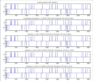
In a general compressed sensing model, we set the hits of a signalx∈RNisN= . There existm= spikes with amplitude± distributed in the whole domain randomly. The plot can be seen on the top of Figure . Then we set the observation dimensionM= and a
matrixAwithM×Norder is also generated arbitrarily. A standard Gaussian distribution noise with varianceσε= –is added. Lett= in (.).
For the step sizes (.) and (.), we always set the constantρ= . For Algorithm ., we setβn= .. All the processes are started with initial signalx= and finished with the
stop rule
xn+–xn/xn< –.
We calculated the mean squared error (MSE) for the results
MSE= (/N)x∗–x,
wherex∗is an estimated signal ofx.
The second and third plots in Figure correspond to the results with step sizes (.) and (.) to Algorithm ., respectively. The recovered result by Algorithm . with step size (.) is shown in the fourth plot. Especially for the fifth, when we setβn= (n+ )–k, k= , , , . . . , when we havek≥ the iteration steps of Algorithm . start to approach the number in the second plot, and the restored precision is a little poorer than the others. For (.) we firstly setσn=σ= .; then in order to study its effect to the convergence
speed of the CQ algorithm, we let it beσn= (n+ )–l,l≥ is an integer. In Figure we
can find that whenl≥ the best MSE curves can be obtained, and it starts to change less. Therefore,σnshould be as little as possible.
4.2 Image deconvolution
In this subsection, we continue by applying Algorithms . and . to recover the blurred Cameraman image. In the experiments, from [, ] we employ Haar wavelets and the blur point spread functionhij= ( +i+j)–, fori,j= –, . . . , ; the noise variance isσ= .
The size of the image isN=M= . The threshold value is hand-tuned for the best SNR
improvement.tis the sum of all the original pixel values.
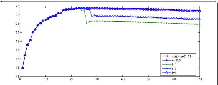
We observe the performance ofσnin (.); see Figure . We find that at the beginning
several steps there are similar SNR curves, however, after iterations,σ= . is similar with (.). When ≤l< , the curves are worse than the others. While we setl≥ the curve starts to be consistent with the curve of (.). Therefore, we also know that σn
Figure 1 Compressed sensing problem, from top to bottom: original signal, results of CQ algorithm with step sizes (1.11), (1.12), and Algorithm 3.3.
Figure 2 The performance curves of MSE to differentσnin 100 iterations.The line with squares is
corresponding toσn= 0.5,xcorresponding tol=1, circles tol=4, points tol=16.
5 Conclusion remarks
In this paper we have proposed several kinds of adaptively relaxed iterative algorithms with a new variable step sizeτnfor solving SFP (.). The feature is that the new variable
step sizeτncontains a sequence of positive numbers in its denominator. Because of this,
[image:20.595.116.478.430.583.2]Figure 3 The performance curves of SNR to differentσnin 70 iterations.The line with squares
corresponds to (1.11),xtol= 1, triangles tol= 3, circles tol= 16.
By means of new analysis techniques, we have proved several kinds of weak and strong convergence theorems of the proposed algorithms for solving SFP (.), which improved, extended, and complemented those existing in the literature. We remark that all conver-gence results in this paper still hold true if we use the step sizeτngiven by (.) to replace
the step size given by (.). In such a case, the stop rules should be modified. We would like to point out that our Theorems . and . are closely related to a sort of variational inequalities.
Finally, numerical experiments have been presented to illustrate the effectiveness of the proposed algorithms and applications in signal processing of the algorithms with the step size selected in this paper. The numerical results tell us that the changes of the choice of the step sizeσngiven by (.) may affect the convergence rate of the iterative algorithms,
andσnshould be chosen as small as possible; for instance, we can chooseσnsuch that
σn→ asn→ ∞.
Competing interests
The authors declare that they have no competing interests.
Authors’ contributions
All the authors contributed equally. All authors read and approved the final manuscript.
Author details
1Department of Mathematics and Information, Hebei Normal University, Shijiazhuang, 050024, China.2Department of
Mathematics, Shijiazhuang Mechanical Engineering College, Shijiazhuang, 050003, China.3The Second Training Base,
Naval Aviation Institution, Huludao, 125001, China.
Acknowledgements
This research was supported by the National Natural Science Foundation of China (11071053).
Received: 26 February 2014 Accepted: 20 October 2014 Published:05 Nov 2014 References
1. Censor, Y, Elfving, T: A multiprojection algorithm using Bregman projections in a product space. Numer. Algorithms8, 221-239 (1994)
2. López, G, Martín-Márquez, V, Xu, HK: Iterative algorithms for the multiple-sets split feasibility problem. In: Censor, Y, Jiang, M, Wang, G (eds.) Biomedical Mathematics: Promising Directions in Imaging, Therapy Planning and Inverse Problems, pp. 243-279. Medical Physics Publishing, Madison (2009)
3. Chang, SS, Kim, JK, Cho, YJ, Sim, JY: Weak and strong convergence theorems of solutions to split feasibility problem for nonspreading type mapping in Hilbert spaces. Fixed Point Theory Appl.2014, Article ID 11 (2014)
4. Stark, H, Yang, Y: Vector Space Projections: a Numerical Approach to Signal and Image Processing, Neural Nets and Optics. Wiley, New York (1998)
6. Censor, Y, Elfving, T, Kopf, N, Bortfeld, T: The multiple-sets split feasibility problem and its applications for inverse problems. Inverse Probl.21, 2071-2084 (2005)
7. Qu, B, Xiu, N: A note on the CQ algorithm for the split feasibility problem. Inverse Probl.21, 1655-1665 (2005) 8. Li, M: Improved relaxed CQ methods for solving the split feasibility problem. Adv. Model. Optim.13, 305-318 (2011) 9. Abdellah, B, Muhammad, AN, Mohamed, K, Sheng, ZH: On descent-projection method for solving the split feasibility
problems. J. Glob. Optim.54, 627-639 (2012)
10. Yang, Q: On variable-step relaxed projection algorithm for variational inequalities. J. Math. Anal. Appl.302, 166-179 (2005)
11. López, G, Martín-Márquez, V, Wang, FH, Xu, HK: Solving the split feasibility problem without prior knowledge of matrix norms. Inverse Probl.28, 085004 (2012)
12. Göebel, K, Kirk, WA: Topics on Metric Fixed Point Theory. Cambridge University Press, Cambridge (1990) 13. Aubin, JP: Optima and Equilibria: An Introduction to Nonlinear Analysis. Springer, Berlin (1993)
14. Byrne, C: A unified treatment of some iterative algorithms in signal processing and image reconstruction. Inverse Probl.20, 103-120 (2004)
15. Bauschke, HH, Borwein, JM: On projection algorithms for solving convex feasibility problems. SIAM Rev.38, 367-426 (1996)
16. Xu, HK: Iterative algorithms for nonlinear operators. J. Lond. Math. Soc.66, 240-256 (2011)
17. Wang, FH, Xu, HK: Approximating curve and strong convergence of the CQ algorithm for the split feasibility problem. J. Inequal. Appl. (2010). doi:10.1155/2010/102085
18. Dang, YZ, Gao, Y: The strong convergence of a KM-CQ-like algorithm for a split feasibility problem. Inverse Probl.27, 015007 (2011)
19. Yu, X, Shahzad, N, Yao, YH: Implicit and explicit algorithms for solving the split feasibility problem. Optim. Lett.6, 1447-1462 (2012)
20. Yao, YH, Postolache, M, Liou, YC: Strong convergence of a self-adaptive method for the split feasibility problem. Fixed Point Theory Appl.2013, Article ID 201 (2013). doi:10.1186/1687-1812-2013-201
21. Daubechies, I, Fornasier, M, Loris, I: Accelerated projected gradient method for linear inverse problems with sparsity constraints. J. Fourier Anal. Appl.14, 764-792 (2008)
22. Figueiredo, MA, Nowak, RD, Wright, SJ: Gradient projection for sparse reconstruction: application to compressed sensing and other inverse problems. IEEE J. Sel. Top. Signal Process.1, 586-598 (2007)
23. Starck, JL, Murtagh, F, Fadili, JM: Sparse Image and Signal Processing Wavelets, Curvelets, Morphological Diversity, p. 166. Cambridge University Press, Cambridge (2010)
24. Mário, ATF: An EM algorithm for wavelet-based image restoration. IEEE Trans. Image Process.12, 906-917 (2003)
10.1186/1029-242X-2014-448