Component Safety Assessment Using Three State Markov Chain Model

© 2015, IRJET ISO 9001:2008 Certified Journal

Page 299

COMPONENT SAFETY ASSESSMENT USING THREE-STATE MARKOV

CHAIN MODEL

Gandi Satyanarayana

_{, Dr. P. Seetharamaiah}

1

_{Research Scholar}

_{, Computer Science & Engineering, GITAM University, AndhraPradesh, India}

1

_{Professor Emeritus}

_{, Computer Science& System Engineering, Andhra University, AndhraPradesh, India}

order to model both design faults and physical faults through a three-state homogenous Markov model that is used to solve three state non homogeneous Markov chain for the component modeling. Four parameters are used in the modeling of the three-state Markov chain model. By using the parameterized three-state Markov model Component safety assessment is conducted by the assumption that component does not utilize redundancy.

Key Words:

Safety-critical computer systems, Faults,

hazard, Errors, Failures, Physical Fault, Design

Failures, Safe Failures, Unsafe Failures, Coverage,

Failure rate,

1. Introduction

Safety-critical system and computer system are the two concepts concerned in a safety critical computer system. A safety-critical system is a system whose faulty function could have very serious effects such as the loss of severe injuries, large-scale environmental spoil, human life, or large cost-effective penalties, A computer system [IEEE 729] is a system composed of computer, peripherals, and the software essential to make them work together. Here we deal with component modeling and assessment. A system is comprised of at least one component. The assumption in modeling of components is that component does not utilize redundancy. A simplex system is a system that does not utilize redundancy frequently. [Dunn2002]. Redundancy is the usage of additional resources further than those needed for the normal system operation for the purpose of achieving fault tolerance [Johnsonl989]. Fault tolerance is the ability of a system to continue to perform its tasks properly during and after the occurrence of hardware and/or software faults [Johnson 1989]. For example, in Triple Modular Redundancy (TMR), a typical fault tolerant design is achieved through three redundant components.

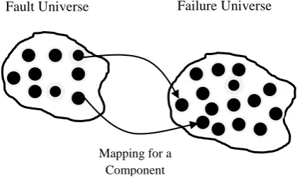
A system can be designed with both fault tolerant mechanisms and fault detection mechanisms. A component cannot have any fault tolerant mechanisms, but a component can have fault detection mechanisms. Actually Components are the building blocks of a system. By the assumption that a component is non-redundant, the fault universe and the failure universe of a component is a one-to-one mapping, as shown in Figure 1-1.

Figure 1-1 Component Fault-Failure Mapping

1-1 Hazard, Faults, Errors and Failures

A system may not always achieve the desired aim .The factors of reliability of a system arises due to causes and effects of deviation from the system functioning. The following definitions come from [N.G.Leveson 2001]. Definition 1.1: Hazard is the potential to cause harm to people, Environment, Asset and Reputation of an organization.

Definition 1.2: Fault is a physical defect, imperfection, or flaw that occurs within some hardware or software component.

Definition 1.3: Error is a design flaw or deviation from a desired or intended state.

Definition 1.4: Failure is the non-performance or inability of a system or component to perform its intended function for a specified time under specified environmental conditions.

Mapping for a Component

© 2015, IRJET ISO 9001:2008 Certified Journal

Page 300

1.2 List of Notations

F Fault space

Ω Failure rate

ΩP Physical Fault failure rate

ΩD Design fault failure rate

ΩXP Physical fault failure rate of X

ΩXD Design fault failure rate of X

Ω (t) Failure rate of function

Ωij Rate of a transition process makes from state i

into state j ψ State space Φ Repair rate

Ŧ Transition rate matrix

Β Upper case of a letter represents a three-valued Variable

€ Coverage Space

PO (t) Probability of the system stays at operation state

at t

PFS (t) Probability that system stays at fail-safe state at t

PFU (t) Probability that system stays at fail-unsafe state at

t S(t) Safety

SSS Steady-State Safety

2. Problem Statement

A component’s failure rate is decided by the design fault failure rate and the physical fault failure rate with the non-redundancy assumption. Let a design fault failure rate of a component is regarded as statistically non-increasing as a function of time, ΩD(t ) and a physical fault failure rate of a

component is constant, Ωp. Figure 2-1 shows the discrete failure rate function of a component, Ω t =ΩD t +ΩP,

given that the design fault failure rate is updated either periodically or when a design fault is fixed.

Figure 2-1 Failure Rate Function

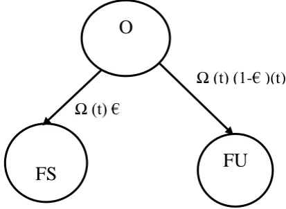
Welke [Welkel995] proposed a unified model, which incorporates the time-varying software failure intensity of the Goel-Okumoto’s NHPP model into the Markov hardware reliability model. Here, the implementation of the Goel- Okumoto model is based on the concept of the rah-order inter-arrival times [Welkel995], and the time varying failure rate needs the transition matrix to be recalculated before each successive matrix multiplication [Welke1988]. In order to quantitatively assess safety, a three-state Markov model is built with a failure rate function and a coverage function, which are both time variant, as shown in Figure 2-2.

Markov chain models with time varying transition rates are known as non-homogenous Markov chain models. A time variant coverage is because of the impact of updates on design fault failure rate that will be explained in Corollary 2.1. In most of the cases, the impact can be ignored and the coverage is assumed to be constant. Coverage is time variant or assumed constant, the time variance of the failure rate determines the three-state Markov model to be non-homogenous.

Figure 2-2 Non-Homogenous Three-State Markov Model Solving this Markov chain, we can obtain the probabilities associated with each state:

P

t = e

t

0

PFS t = Ω t 1 − e− Ω Ί dΊ t

0 ₊ dΩ Ί dΊ . e

− Ω Ί dΊ₀t t

0 dΊ

2-2

PFU t = 1 − Ω t 1 − e− Ω Ί dΊ t

0 ₊ dΩ Ί dΊ . e

− Ω Ί dΊ₀t t

0 dΊ

O

FS

FU

Ω (t) €

(t)

Ω (t) (1-€ )(t)

Ω

€

Ί

t

O

FSi+1

FU

Ω(t)

t

Ί2 Ίi Ίj

Ί1

Ω1

Ωi

Ωj

Ω2

© 2015, IRJET ISO 9001:2008 Certified Journal

Page 301

2-3

The three state probabilities have the closed-form solutions that are subject to the formats of the failure rate function Ω (t) and the coverage function € (t). However, the analytic expressions of time variant Ω (t)and € (t) are very difficult, but possible, to obtain. So the problem is to find an engineering solution with appropriate assumptions for the three-state non-homogenous Markov chain model shown in Figure 2-2.

3. Component Safety Assessment

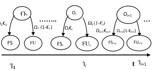
In the Projection of future failure behavior we assume that the model parameter values will not change during the period of projection [Musal999]. If no faults are introduced or removed, and no operational profile changes have occurred, the failure intensity will be constant [Musal999]. By using this idea, we propose a stepwise solution for the non-homogenous Markov model, as shown in Figure 3-1.

……..

…

Figure 3-1 Piecewise Solution for Non-Homogenous Markov Model

Let us assume ΩD and €D are constant between design

changes. We re-estimate the model parameters using a selected estimation model whenever design changes are made, such as one of the exponential failure time models. With the help of a constant operational profile, ΩDand €D

can be updated when a design fault is removed or a design update is made. After each and every update of parameters, a three-state homogeneous Markov model with the updated parameters can be built, t denotes the time passed since the testing begins, and Ίi, denotes the

time when a design update is made. After each design update, the component is returned to the operational state and starts a new lifecycle. If there is no new update since Ίi, for t > Ίi .We will get the state probability information:

P

t

Ί

= e

3-1

P

t

Ί

= €

(1 − e

)

3-2

P

t

Ί

= (1 − €

) 1 − e

3-3

Suppose Ίi+1 denotes the tie of the (i + 1)th design update

and there is no design update between Ίi , and Ίi+1 .

PO tΊi ,PFS tΊi , and PFU tΊi planned using €, and Ωi are

valid during 1< t < Ίi+1. When there is a conduction of

parameter update at Ίi+1, the three-state Markov model is

refreshed with the updated failure rate Ωi+1 and coverage

€i+1 . PO tΊi+1 ,PFS tΊi+1 , and PFU tΊi+1 can be obtained

and is valid until the next update. So when we observe the component at anytime between updates, we can use a homogenous Markov model to model the component. A three-state homogeneous Markov model shown in Figure 3-2 can be constructed to estimate a component’s fail-safe probability and fail-unsafe probability between design updates or design fault eliminations. Here, the failure rate and the coverage refer to those of a component for a certain period of time when there is no design update and no fault elimination. The following assumptions are made for the proposed approach to determine the component safety.

Assumptions:

1) After a design update, the component starts a new lifecycle. The homogenous Markov model is used between design updates.

2) Let the physical fault failure rate Ωp, the design fault failure rate ΩD, the physical fault coverage

€p, and the design fault coverage €D, are assumed

constant between design updates or eliminations of design faults.

3) Repairs of failures are not modeled caused by physical faults.

By the Assumptions 1 and 3, the repair rate from the fail-safe state to the operational state is zero and is therefore ignored in the model. Because of the consequences of an unsafe failure usually make the component irreparable, the repair rate from the fail-unsafe state to the operational state is zero and ignored in the model. So, repairs are not modeled in the three-state Markov model shown in Figure 3-2.

Ω1 (1-€1)

FU

1

Ωi€i

Ωi (1-€i)

FSi

\

FUi

Ωi+1€i+1 Ωi+1(1-€i+1)

Ί

Ί

t

Ί

FS

1

Oi Oi+1

FSi+1 FUi+1

Ω1€1

© 2015, IRJET ISO 9001:2008 Certified Journal

Page 302

Figure 3-2 Three-State Homogenous Markov Model without Repair

A component’s coverage is dependent on the four parameters: the physical fault failure rate, the physical fault coverage, the design fault failure rate, and the design fault coverage. Corollary 4.1 proves the analytic expression of a component’s coverage given the four parameters. Coverage is the critical parameter for the safety assessment. Thus, Corollary 3.1 lays the foundation for the quantitative safety assessment with the consideration of both physical faults and design faults.

Corollary 3.1.

Let the physical fault failure rate is Ωp, the design fault failure rate is ΩD, the physical fault coverage is €P, and the

design fault coverage is €D between two design updates.

Then the coverage of the component between the two updates is given in the following equation:

€= _ΩΩD

D+Ω_P .€D+ ΩP

Ω_D+Ω_D .€P 3-4

Proof.

The total of two independent Poisson processes is still a Poisson process. The transition rate of the new process is the total of the rates of the two independent Poisson process. Thus, the failure rate of the Markov chain model shown in Figure 3-2 is

Ω=€DΩD+€PΩP+ 1−€D ΩD+ 1−€P ΩP=ΩD+ΩP

3-5

Then the transition rate from the operation state to the fail-safe state is €DΩD + €PΩP.

Given Corollary 2.1, the analytic expression of coverage is derived in the following equation.

€=€DΩD+€PΩP

ΩD+ΩP =

ΩD

ΩD+ΩP€D+

ΩP

ΩD+ΩP€P

3-6

■

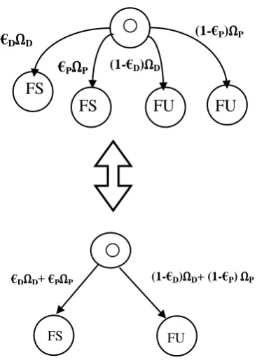
According to Corollary 3.1, a three-state homogeneous Markov model between design updates can be constructed with the constant failure rate, ΩD +ΩP, and the constant

coverage, ΩD

ΩD+ΩP €D+ ΩP

ΩD+ΩP €P as shown in Figure 3-3.

Figure 3-3 Three-State Homogenous Markov Model By using the four parameters of the Markov chain model shown in Figure 3-3, we can express the probabilities associated with each state using the following equations. PO=e− ΩD+ΩPt

3-7 PFS= €D_ΩΩD+€PΩP

D+Ω_P −

€_DΩ_D+€_PΩ_P Ω_D+Ω_P e

− Ω_D+Ω_P t

3-8 PFU=

(1−€_D)ΩD+(1−€P)Ω_P ΩD+ΩP −

(1−€_D)Ω_D+ 1−€PΩP ΩD+ΩP e

− ΩD+ΩPt

3-9 Let us recall that safety is the sum of the probability that a system stays in the operational State at t, that is also the reliability of the modeled system R (t), and the probability that a system goes to the fail-safe state by t. Thus,

€

Ω

€

Ω

(1-€P)ΩP

€DΩD+ €PΩP (1-€D)ΩD+ (1-€P) ΩP

C

∝

FS

FS

FU

FU

FS _FU

(1-€D)ΩD

FS

_FU

€DΩD+ €PΩP

(1-€D)ΩD+ (1-€P) ΩP

C

∝

FS

FU

© 2015, IRJET ISO 9001:2008 Certified Journal

Page 303

ΩD+ΩP + 1−

€DΩD+€PΩP

ΩD+ΩP e

− ΩD+ΩPt

3-10 And steady-state safety is safety as time approaches infinity.

SSS = lim

t→∞S t = limt→∞

€DΩD+ €PΩP

ΩD+ ΩP

+ 1 −€DΩD+ €PΩP ΩD+ ΩP

e− ΩD+ΩP t

=€DΩD+ €PΩP ΩD+ ΩP

= €

3-11

4. Component MTTUF Assessment

Mean Time To Unsafe Failure (MTTUF) is an significant metric for the assessment of safety-critical systems. It measures the estimated time a system will operate before the first unsafe failure. If the fail-safe state is a repairable state it directly affects the estimated value of the MTTUF. When a failure is caused by a safe fault occurrence; the component goes to the fail-safe state. If the component can be repaired at the fail-safe state, the repair from a failure state to the operational state usually takes some time. Because of the repairs occurred, the component can go to the fail-safe state multiple times before it finally goes to the fail unsafe state.

Definition 4.1: Repair rate μ [Johnsonl989] is the expected number of repairs per unit of time.

The repair rate of a component is calculated by experimental data collected over a period of time. For example, a repair rate can be calculated from a repair log recorded by means of repair technicians. With the repair rate information, the three-state Markov model can be revised to model repairs.

Assumptions:

1) Let the physical fault failure rate ΩP, the design fault

failure rate ΩD, the physical fault coverage €P, and the

design fault coverage €Dare assumed as constant between

design updates or eliminations of design faults. 2) After each repair, the component is perfect as new. 3) Failures caused by unsafe faults are irreparable.

Since the three-state homogenous Markov model shown in Figure 4-1 is valid between design updates or eliminations of design faults, the repairs modeled in the revised three-state Markov model shown in Figure 4-1 do not cause

design alternations or design fault eliminations. An example of these types of repairs is substitute of a worn-out physical part.

μ

Figure 4-1 Three-State Homogenous Markov Model with Repair

When a repair involves a design update or design fault elimination, the homogenous Markov model needs to be solved with updated ΩD and €D for safety and MTTUF

assessment, Ί, represents the time when a design update is made, Ίi+1 denotes the time the next design update is

made. Let us assume there is no design update between Ίt

and Ίi+l. The MTTUF calculated using €i, and Ωiare valid

during Ίi < t < Ίi+1.

……

∞

Figure 4-2 Piecewise Solution for Non-Homogenous Markov Model with Repair

Definition 4.2: MTTF [Johnson 1989] is the expected time that a system will operate before the first failure occurs. Corollary 4.2 proves the analytic expression of a component’s MTTUF given the MTTF and coverage information of the component. Since unsafe failures of safety-critical computer systems are rare events observed in the field, in order to estimate the MTTUF a very long time is usually needed to collect sufficient unsafe failure information. Corollary 4.2 provides a practical approach to estimating the MTTUF.

Corollary 4.2.

FS

_FU

€

Ω

+ €

Ω

(1-€

)

Ω

+

C

∝

FU

Ω€

μ

FS

Ω1 (1-€1)

FU1

Ωi€i Ωi (1-€i)

FSi

\

FUi

Ωi+1€i+1 Ωi+1(1-€i+1)

Ί

Ί

t

Ί

FS1

Oi Oi+1

FSi+1 FUi+1

Ω1€1

O1

μ

μ

© 2015, IRJET ISO 9001:2008 Certified Journal

Page 304

event than a fail-unsafe event and the time only counts the operational time. The MTTUF can be calculated using the following equation:

MTTUF=MTTF₁

−€ 4-1

5. Analysis of Examples

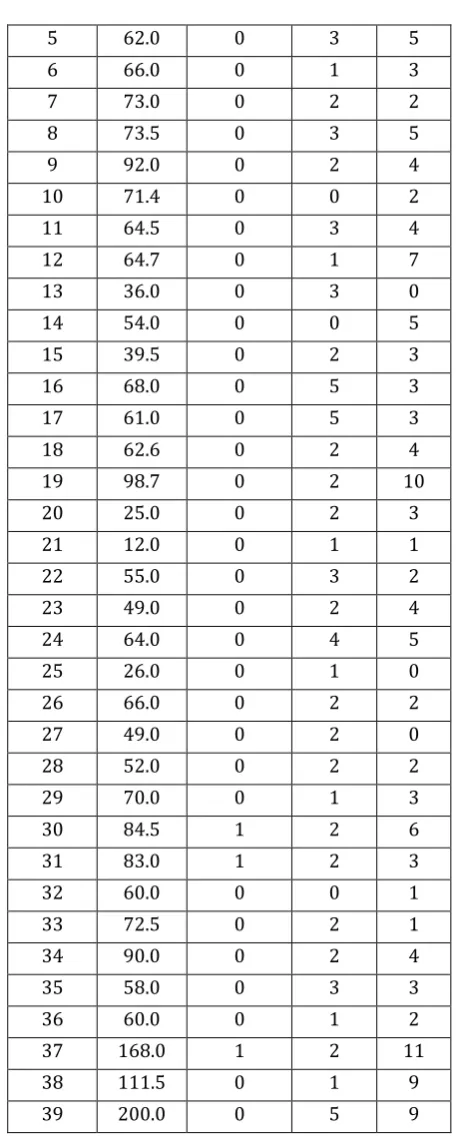
The processing support to exercise command and control over flight operations is given by The Space Shuttle Ground System provides the flight controllers at the Johnson Space Center. Actually the real-time software system of the Space Shuttle Ground System has over one-half million lines of source code. A 2656.9 testing hour record of 39 time intervals was released in [Misra 1983].For the real-time software system the software testing information is provided by the dataset up to 2656.9 hours. Let us consider the real-time software system as one component of the Space Shuttle Ground System, and we perform the quantitative safety assessment for this component. All software faults are considered as design faults. The design fault failure rate and the design fault coverage of the component can be predicted using the information shown in Table 4-1. Let us assume the physical fault failure rate of the real-time software system is zero.

In this Space Shuttle Ground System example, the critical faults are assigned to the unsafe fault subspace and the major faults and the minor faults are assigned to the safe fault subspace. Based on the result of the model goodness-of-fit test The G-O model is selected to model the component. The model’s goodness-of-fit test was conducted with the help of a software package, SM ERFS3, developed by Naval Surface Warfare Center. There are 39 testing intervals in the testing dataset. The design fault failure rate and the design fault coverage can be predicted using the available testing data at the end of each testing interval. So, safety can be estimated by using the parameterized three-state homogeneous Markov model shown in Figure 3-3.Let us assume the time to eliminate a safe fault after it is discovered is small and can be neglected. Thus, MTTUF can be estimated using Equation 4.1.

Interval No.

Test Hours

Critical Faults

Major Faults

Minor Faults

1 62.5 0 6 9

2 44.0 0 2 4

3 40.0 0 1 7

4 68.0 1 1 6

5 62.0 0 3 5

6 66.0 0 1 3

7 73.0 0 2 2

8 73.5 0 3 5

9 92.0 0 2 4

10 71.4 0 0 2

11 64.5 0 3 4

12 64.7 0 1 7

13 36.0 0 3 0

14 54.0 0 0 5

15 39.5 0 2 3

16 68.0 0 5 3

17 61.0 0 5 3

18 62.6 0 2 4

19 98.7 0 2 10

20 25.0 0 2 3

21 12.0 0 1 1

22 55.0 0 3 2

23 49.0 0 2 4

24 64.0 0 4 5

25 26.0 0 1 0

26 66.0 0 2 2

27 49.0 0 2 0

28 52.0 0 2 2

29 70.0 0 1 3

30 84.5 1 2 6

31 83.0 1 2 3

32 60.0 0 0 1

33 72.5 0 2 1

34 90.0 0 2 4

35 58.0 0 3 3

36 60.0 0 1 2

37 168.0 1 2 11

38 111.5 0 1 9

39 200.0 0 5 9

Table 4-1 the Software Fault Dataset of the Space Shuttle Ground System

Example 1: Safety Assessment at t = 2656.9.

© 2015, IRJET ISO 9001:2008 Certified Journal

Page 305

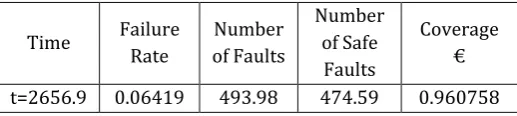
has the ability to estimate the fault content, after the Goel-Okumoto model is applied to the fault dataset shown in Table 4-1 the number of faults is estimated to be 493.98 at t = 2656.9. Inorder to estimate the number of safe faults, the safe fault dataset is needed and it can be constructed from Table 4-1. Since the major faults and the minor faults are assigned to the safe fault subspace, the information of the major faults and the minor faults shown in

Table 4-1 is used to form the safe fault dataset. After the Goel-Okumoto model is applied to the safe fault dataset, the number of safe faults is estimated to be 474.59 at t -

2656.9. Given Equation 3.21, the coverage is predicted to be the ratio of the number of safe design faults to the number of design faults, and the estimated coverage is 0.96075 at t = 2656.9. All statistical calculations were conducted using SMERFS3.

Time Failure Rate

Number of Faults

Number of Safe

Faults

Coverage €

t=2656.9 0.06419 493.98 474.59 0.960758

Table 4-2 Estimated Parameters at t=2656.9 At t=2656.9, the safety of the component is estimated using the following equation:

S t =e−Ωt−2656.9 _{+€ 1−e}−Ωt−2656.9

= 𝑒−0.06419 𝑡−2656.9 _{+0.96075 1− 𝑒}−0.06419 𝑡−2656.9

For example, the estimated safety value at t = 2657.9, one testing hour after the last update, is

S t=2657.9 =e−0.06419_{+0.96075 1−}

e−0.06419) =0-9975597

At t = 2656.9, the MTTUF of the component is estimated to be

MTTUF=MTTF

1−€ = 1 Ω 1−€

= ₀ 1

.064191−0.96075 =396.406

5. Conclusion

In this paper, the approaches to quantitatively assessing safety on components are developed. If no fault introduction, no fault removal, and no operational profile changes are occurring, the failure intensity will be constant [Musa1999]. Using this idea, a piecewise solution, which is based on a

three-state homogenous Markov chain model, is proposed to solve the three-state non-homogenous Markov chain for the component modeling. Corollary 3.1 proves that the analytic expression of a component’s coverage is decided by the four parameters: the physical fault failure rate, the physical fault coverage, the design fault failure rate, and the design fault coverage. A three-state Markov chain without repair model is built to estimate the safety of a component, and a three-state Markov chain with repair model is built to estimate the MTTUF of a component. Using Wald’s Equality, Corollary 4.2 proves that the analytic expression of a component’s MTTUF is decided by the component’s MTTF and the component’s coverage. Both Corollary 4.1 and Corollary 4.2 are important, because they are the foundation of the quantitative safety assessment. A case study is conducted to illustrate the techniques developed in this paper.

References

1.[Anderson81] T. Anderson and P. A. Lee, Fault Tolerance Principles and Practice, Prentice-Hall International, 1981. 2.[Anderson83] T. Anderson and J. C. Knight, A Framework for Software Fault Tolerance in Real-Time Systems, IEEE Transactions On Software Engineering, vol. SE-9, no. 3, pp. 355-364, 1983.

3.[Anderson08] Paul Anderson, Detecting Bugs in Safety Critical Code , Dr. Dobbs Journal, February, 2008 [Avizienis76] A. Avizienis, Fault Tolerant Systems, IEEE Transactions On Computers, vol. C-25, pp. 1304- 1312, 1976.

4.[Bedford01] T. Bedford and R. Cooke, Probabilistic Risk Analysis: Foundations and Methods, Cambridge Univ. Press, 2001.

5. J. V. Bukowski and W. M. Goble, “Defining mean time-to-failure in a particular time-to-failure-state for multi-time-to-failure-state systems,” IEEE Trans. Reliab.,

vol. 50, no. 2, pp. 221–228, Jun. 2001.

6.C. Y. Choi, B. W. Johnson, and J. A. Profeta III, “Safety issues in the comparative analysis of dependable architectures,” IEEE Trans. Reliab., vol. 46, no. 3, pp. 316– 322, Sep. 1997.

© 2015, IRJET ISO 9001:2008 Certified Journal

Page 306

28, 1993, pp. 55–63.

8 W. M. Goble, Control Systems Safety Evaluation and Reliability: Instrument Society of America, 1998.

9. IEEE 100, “The Authoritative Dictionary of IEEE Standard Terms,”

IEEE Press, 2000.

10.[A rlatl990] Arlat, J., Y. Crouzet, and J.-C. Laprie, “Fault Injection for the Experimental Validation of Fault Tolerance,” LAAS Report 90415,1990.

11.[A vizienisl982] Avizienis, A., “The Four-Universe Information System Model for the Study of Fault Tolerance,” Proceedings of the 12th Annual International Symposium on Fault-Tolerant Computing, June 1982, pp. 6-13.

12.[Bowen2000] Bowen, J., “The Ethics of Safety-Critical Systems,” Communications of ACM, Vol. 43, Issue 4, 2000, pp. 91-97.

13.[Bishop 1998] Bishop, Peter, R. Bloomfield, “A methodology for Safety Case Development,” Proceedings of the Sixth Safety-critical Systems Symposium, February 1998.

14.[C arterl969] Bouricius, W .G., W.C. Carter, and P.R. Schneider, “Reliability Modeling Techniques for Self-repairing Computer Systems,” 24th Annual ACM National conference, 1969, pp. 295-309.

15.[Ciardol993] Ciardo, G., and K. S. Trivedi, “A Decomposition Approach for Stochastic Reward Net models,” Performance Evaluation, Vol. 18, No. 1, 1993, pp. 37-59.

16.[Courtoisl977] P. J. Courtois, Decomposability: Queuing and Computer System Applications, Academic Dress, New York, 1977.

17.[D aehnl991] Daehn, Wilfried, “Fault Injection Using Small Fault Samples,” Journal of Electronic Testing: Theory and Applications, Vol. 2, 1991, p p.191-203.

18.[DFWCS1] Digital Feed-Water Software Revision Log, December 2005.

19.[Medikonda10] Ben Medikonda M. and

P.Seetharamaiah, Integrated Safety Analysis of Software-Controlled Critical Systems, ACM SIGSOFT Software Engineering Notes (SEN), Volume 35, Number 1, January 2010, p.36.

20.[NASA8719] NASA Software Safety Guidebook, STD-8719-13A, NASA Glenn Research Center, Safety and Assurance Directorate

21.[Online]http://www.hq.nasa.gov/office/ codeq/ doctree/ 871913.pdf [2007 June 12].

22.[NATO4404] NATO Standardization Agreement (STANAG) 4404 Safety Design Requirements and Guidelines for Munitions Related Safety Critical Computing Systems, 1996.

23.[NUREG0492] Fault Tree Handbook, NUREG-0492, US Nuclear Regulatory Commission,1981,www.nrc.gov/

reading - rm/ doc-collections / nuregs / staff / sr0492 / sr0492. pdf.

24.[Neumann91] P. G. Neumann, The Computer-Related Risk of the Year:Weak Links and Correlated Events, Proceedings of the Sixth Annual Conference on Computer Assurance. NIST/IEEE, 1991, pp.5-8. 25.[Neumann95] Neumann, Peter G., Computer Related Risks Addison-Wesley 1995.