Loss Distributions

Munich Personal RePEc Archive

Loss Distributions

Burnecki, Krzysztof and Misiorek, Adam and Weron, Rafal

2010

Online at

https://mpra.ub.uni-muenchen.de/22163/

Loss Distributions

1

Krzysztof Burnecki

_{, Adam Misiorek}

_{, Rafał Weron}

a_{Hugo Steinhaus Center, Wrocław University of Technology, 50-370 Wrocław, Poland} b_{Institute of Organization and Management, Wrocław University of Technology, 50-370 Wrocław, Poland}

c_{Santander Consumer Bank S.A., Wrocław, Poland}

Abstract

This paper is intended as a guide to statistical inference for loss distributions. There are three basic approaches to deriving the loss distribution in an insurance risk model: empirical, analytical, and moment based. The empirical method is based on a sufficiently smooth and accurate estimate of the cumulative distribution function (cdf) and can be used only when large data sets are available. The analytical approach is probably the most often used in practice and certainly the most frequently adopted in the actuarial literature. It reduces to finding a suitable analytical expression which fits the observed data well and which is easy to handle. In some applications the exact shape of the loss distribution is not required. We may then use the moment based approach, which consists of estimating only the lowest characteristics (moments) of the distribution, like the mean and variance.

Having a large collection of distributions to choose from, we need to narrow our selection to a single model and a unique parameter estimate. The type of the objective loss distribution can be easily selected by comparing the shapes of the empirical and theoretical mean excess functions. Goodness-of-fit can be verified by plotting the corresponding limited expected value functions. Finally, the hypothesis that the modeled random event is governed by a certain loss distribution can be statistically tested.

Keywords: Loss distribution, Insurance risk model, Random variable generation, Goodness-of-fit testing, Mean

excess function, Limited expected value function.

1. Introduction

The derivation of loss distributions from insurance data is not an easy task. Insurers normally keep data files containing detailed information about policies and claims, which are used for accounting and rate-making purposes. However, claim size distributions and other data needed for risk-theoretical analyzes can be obtained usually only after tedious data preprocessing. Moreover, the claim statistics are often limited. Data files containing detailed information about some policies and claims may be missing or corrupted. There may also be situations where prior data or experience are not available at all, e.g. when a new type of insurance is introduced or when very large special risks are insured. Then the distribution has to be based on knowledge of similar risks or on extrapolation of lesser risks.

There are three basic approaches to deriving the loss distribution: empirical, analytical, and moment based. The empirical method, presented in Section 2, can be used only when large data sets are available. In such cases a sufficiently smooth and accurate estimate of the cumulative distribution function (cdf) is obtained. Sometimes the application of curve fitting techniques – used to smooth the empirical distribution function – can be beneficial. If the curve can be described by a function with a tractable analytical form, then this approach becomes computationally efficient and similar to the second method.

The analytical approach is probably the most often used in practice and certainly the most frequently adopted in the actuarial literature. It reduces to finding a suitable analytical expression which fits the observed data well and which is easy to handle. Basic characteristics and estimation issues for the most popular and useful loss distributions

are discussed in Section 3. Note, that sometimes it may be helpful to subdivide the range of the claim size distribution into intervals for which different methods are employed. For example, the small and medium size claims could be described by the empirical claim size distribution, while the large claims – for which the scarcity of data eliminates the use of the empirical approach – by an analytical loss distribution.

In some applications the exact shape of the loss distribution is not required. We may then use the moment based approach, which consists of estimating only the lowest characteristics (moments) of the distribution, like the mean and variance. However, it should be kept in mind that even the lowest three or four moments do not fully define the shape of a distribution, and therefore the fit to the observed data may be poor. Further details on the moment based approach can be found e.g. in Daykin, Pentikainen, and Pesonen (1994).

Having a large collection of distributions to choose from, we need to narrow our selection to a single model and a unique parameter estimate. The type of the objective loss distribution can be easily selected by comparing the shapes of the empirical and theoretical mean excess functions. Goodness-of-fit can be verified by plotting the corresponding limited expected value functions. Finally, the hypothesis that the modeled random event is governed by a certain loss distribution can be statistically tested. In Section 4 these statistical issues are thoroughly discussed.

In Section 5 we apply the presented tools to modeling real-world insurance data. The analysis is conducted for two datasets: (i) the PCS (Property Claim Services) dataset covering losses resulting from catastrophic events in USA that occurred between 1990 and 1999 and (ii) the Danish fire losses dataset, which concerns major fire losses that occurred between 1980 and 1990 and were recorded by Copenhagen Re.

2. Empirical distribution function

A natural estimate for the loss distribution is the observed (empirical) claim size distribution. However, if there have been changes in monetary values during the observation period, inflation corrected data should be used. For a sample of observations{x1, . . . ,x_n}the empirical distribution function (edf) is defined as:

Fn(x)=

1

n#{i:xi≤x}, (1)

i.e. it is a piecewise constant function with jumps of size 1/n at pointsxi. Very often, especially if the sample is

large, the edf is approximated by a continuous, piecewise linear function with the “jump points” connected by linear functions, see Figure 1.

The empirical distribution function approach is appropriate only when there is a sufficiently large volume of claim data. This is rarely the case for the tail of the distribution, especially in situations where exceptionally large claims are possible. It is often advisable to divide the range of relevant values of claims into two parts, treating the claim sizes up to some limit on a discrete basis, while the tail is replaced by an analytical cdf.

3. Analytical methods

It is often desirable to find an explicit analytical expression for a loss distribution. This is particularly the case if the claim statistics are too sparse to use the empirical approach. It should be stressed, however, that many standard models in statistics – like the Gaussian distribution – are unsuitable for fitting the claim size distribution. The main reason for this is the strongly skewed nature of loss distributions. The log-normal, Pareto, Burr, Weibull, and gamma distributions are typical candidates for claim size distributions to be considered in applications.

3.1. Log-normal distribution

Consider a random variableXwhich has the normal distribution with density

fN(x)=

1

√

2πσexp

(

−1

2

(x₋µ)2

σ2

)

, _−∞<x<_∞. (2)

LetY =eX_{so thatX=logY. Then the probability density function ofYis given by:}

f(y)= fN(logy)

1

y =

1

√

2πσyexp

(

−1

2

(logy₋µ)2

σ2

)

0 0.5 1 1.5 2 2.5 3 3.5 4 0 0.1 0.2 0.3 0.4 0.5 0.6 0.7 0.8 0.9 1

Empirical distribution function

x

CDF(x)

0 1 2 3 4 5

0 0.1 0.2 0.3 0.4 0.5 0.6 0.7 0.8 0.9 1

Empirical and lognormal distributions

x

CDF(x)

Figure 1:Left panel: Empirical distribution function (edf) of a 10-element log-normally distributed sample with parametersµ=0.5 andσ=0.5, see Section 3.1.Right panel: Approximation of the edf by a continuous, piecewise linear function (black solid line) and the theoretical distribution function (red dotted line).

whereσ > 0 is the scale and−∞ < µ < _∞is the location parameter. The distribution ofY is termed log-normal, however, sometimes it is called the Cobb-Douglas law, especially when applied to econometric data. The log-normal cdf is given by:

F(y)= Φ logy−µ

σ

!

, y>0, (4)

whereΦ(·) is the standard normal (with mean 0 and variance l) distribution function. Thek-th raw momentmkof the

log-normal variate can be easily derived using results for normal random variables:

mk=E

Yk=EekX=MX(k)=exp µk+

σ2_k2

2

!

, (5)

whereMX(z) is the moment generating function of the normal distribution. In particular, the mean and variance are

E(X) = exp µ+σ 2

2

!

, (6)

Var(X) = nexpσ2₋1oexp2µ+σ2, (7) respectively. For both standard parameter estimation techniques the estimators are known in closed form. The method of moments estimators are given by:

ˆ

µ = 2 log

       1 n n X i=1 xi       − 1 2log        1 n n X i=1

x2_i

     

, (8)

ˆ

σ2 = log

       1 n n X i=1

x2_i

      −2 log

       1 n n X i=1 xi        , (9)

while the maximum likelihood estimators by:

ˆ

µ = 1 n

n

X

i=1

log(xi), (10)

ˆ

σ2 = 1 n

n

X

i=1

0 5 10 15 20 25 0

0.1 0.2 0.3 0.4 0.5

x

PDF(x)

Log−normal densities

0 1 2 3 4 5 6 7 8

0 0.2 0.4 0.6 0.8 1 1.2 1.4 1.6

x

PDF(x)

Exponential densities

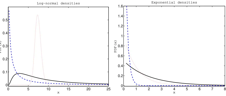
Figure 2:Left panel:Log-normal probability density functions (pdfs) with parametersµ=2 andσ=1 (black solid line),µ=2 andσ=0.1 (red dotted line), andµ=0.5 andσ=2 (blue dashed line).Right panel:Exponential pdfs with parameterβ=0.5 (black solid line),β=1 (red dotted line), andβ=5 (blue dashed line).

Finally, the generation of a log-normal variate is straightforward. We simply have to take the exponent of a normal variate.

The log-normal distribution is very useful in modeling of claim sizes. It is right-skewed, has a thick tail and fits many situations well. For smallσit resembles a normal distribution (see the left panel in Figure 2) although this is not always desirable. It is infinitely divisible and closed under scale and power transformations. However, it also suffers from some drawbacks. Most notably, the Laplace transform does not have a closed form representation and the moment generating function does not exist.

3.2. Exponential distribution

Consider the random variable with the following density and distribution functions, respectively:

f(x) = βe−βx, x>0, (12)

F(x) = 1−e−βx, x>0. (13)

This distribution is termed an exponential distribution with parameter (or intensity)β >0. The Laplace transform of (12) is

L(t)def=

Z ∞

0

e−txf(x)dx= β

β+t, t>−β, (14)

yielding the general formula for thek-th raw moment

mk

def = (−1)k∂

k_L(t)

∂tk

_t=0 =

k!

βk. (15)

The mean and variance are thusβ−1_andβ−2_{, respectively. The maximum likelihood estimator (equal to the method of}

moments estimator) forβis given by:

ˆ

β= 1

ˆ

m1

, (16)

where

ˆ

mk=

1

n n

X

i=1

is the samplek-th raw moment.

To generate an exponential random variableXwith intensityβwe can use the inverse transform method (L’Ecuyer, 2004; Ross, 2002). The method consists of taking a random numberUdistributed uniformly on the interval (0,1) and settingX = F−1_{(U), whereF}−1_{(x) =}

−1βlog(1−x) is the inverse of the exponential cdf (13). In fact we can set

X=₋1_βlogUsince 1−Uhas the same distribution asU.

The exponential distribution has many interesting features. For example, it has the memoryless property, i.e. P(X >x+y_|X >y) =P(X > x). It also arises as the inter-occurrence times of the events in a Poisson process, see Chapter 14 in Ciˇzek, H¨ardle, and Weron (2005). Then-th root of the Laplace transform (14) is

L(t)= β

β+t

!1_n

, (18)

which is the Laplace transform of a gamma variate (see Section 3.6). Thus the exponential distribution is infinitely divisible.

The exponential distribution is often used in developing models of insurance risks. This usefulness stems in a large part from its many and varied tractable mathematical properties. However, a disadvantage of the exponential distribution is that its density is monotone decreasing (see the right panel in Figure 2), a situation which may not be appropriate in some practical situations.

3.3. Pareto distribution

Suppose that a variateXhas (conditional onβ) an exponential distribution with meanβ−1_{. Further, suppose that}

βitself has a gamma distribution (see Section 3.6). The unconditional distribution ofXis a mixture and is called the Pareto distribution. Moreover, it can be shown that ifXis an exponential random variable andYis a gamma random variable, thenX/Yis a Pareto random variable.

The density and distribution functions of a Pareto variate are given by:

f(x) = αλ

α

(λ+x)α+1, x>0, (19)

F(x) = 1−

_λ

λ+x

α

, x>0, (20)

respectively. Clearly, the shape parameterαand the scale parameterλare both positive. Thek-th raw moment:

mk=λkk!

Γ(α₋k)

Γ(α) , (21)

exists only fork< α. In the above formula

Γ(a)def=

Z ∞

0

ya−1e−ydy, (22)

is the standard gamma function. The mean and variance are thus:

E(X) = λ

α₋1, (23)

Var(X) = αλ 2

(α₋1)2_(α

−2), (24)

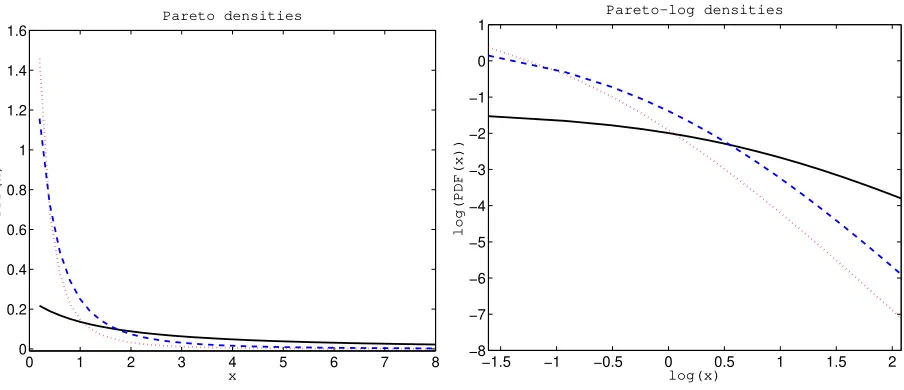
respectively. Note, that the mean exists only forα >1 and the variance only forα >2. Hence, the Pareto distribution has very thick (or heavy) tails, see Figure 3. The method of moments estimators are given by:

ˆ

α = 2 m2ˆ −mˆ

2 1

ˆ

m2₋2 ˆm2

1

, (25)

ˆ

λ = m1ˆ m2ˆ

ˆ

m2−2 ˆm2₁

0 1 2 3 4 5 6 7 8 0

0.2 0.4 0.6 0.8 1 1.2 1.4 1.6

x

PDF(x)

Pareto densities

−1.5 −1 −0.5 0 0.5 1 1.5 2

−8 −7 −6 −5 −4 −3 −2 −1 0 1

log(x)

log(PDF(x))

Pareto−log densities

Figure 3:Left panel:Pareto pdfs with parametersα=0.5 andλ=2 (black solid line),α=2 andλ=0.5 (red dotted line), andα=2 andλ=1 (blue dashed line). Right panel:The same Pareto densities on a double logarithmic plot. The thick power-law tails of the Pareto distribution are clearly visible.

where, as before, ˆmk is the sample k-th raw moment (17). Note, that the estimators are well defined only when

ˆ

m2−2 ˆm21>0. Unfortunately, there are no closed form expressions for the maximum likelihood estimators and they

can only be evaluated numerically.

Like for many other distributions the simulation of a Pareto variateXcan be conducted via the inverse transform method. The inverse of the cdf (20) has a simple analytical formF−1(x) = λn(1−x)−1/α−1o. Hence, we can set

X =λU−1/α

−1, whereUis distributed uniformly on the unit interval. We have to be cautious, however, whenα

is larger but very close to one. The theoretical mean exists, but the right tail is very heavy. The sample mean will, in general, be significantly lower than E(X).

The Pareto law is very useful in modeling claim sizes in insurance, due in large part to its extremely thick tail. Its main drawback lies in its lack of mathematical tractability in some situations. Like for the log-normal distribution, the Laplace transform does not have a closed form representation and the moment generating function does not exist. Moreover, like the exponential pdf the Pareto density (19) is monotone decreasing, which may not be adequate in some practical situations.

3.4. Burr distribution

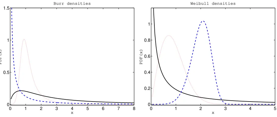
Experience has shown that the Pareto formula is often an appropriate model for the claim size distribution, particu-larly where exceptionally large claims may occur. However, there is sometimes a need to find heavy tailed distributions which offer greater flexibility than the Pareto law, including a non-monotone pdf. Such flexibility is provided by the Burr distribution and its additional shape parameterτ > 0. IfY has the Pareto distribution, then the distribution of

X = Y1/τ_{is known as the Burr distribution, see the left panel in Figure 4. Its density and distribution functions are}

given by:

f(x) = ταλα x

τ−1

(λ+xτ₎α+1, x>0, (27)

F(x) = 1−

_λ

λ+xτ

α

, x>0, (28)

respectively. Thek-th raw moment

mk=

1

Γ(α)λ

k/τ_Γ

1+k

τ

!

Γ α₋k

τ

!

0 1 2 3 4 5 6 7 8 0

0.5 1 1.5

x

PDF(x)

Burr densities

0 1 2 3 4 5

0 0.2 0.4 0.6 0.8 1

x

PDF(x)

Weibull densities

Figure 4:Left panel: Burr pdfs with parametersα=0.5,λ=2 andτ=1.5 (black solid line),α=0.5,λ=0.5 andτ=5 (red dotted line), and

α=2,λ=1 andτ=0.5 (blue dashed line).Right panel:Weibull pdfs with parametersβ=1 andτ=0.5 (black solid line),β=1 andτ=2 (red dotted line), andβ=0.01 andτ=6 (blue dashed line).

exists only fork < τα. Naturally, the Laplace transform does not exist in a closed form and the distribution has no moment generating function as it was the case with the Pareto distribution.

The maximum likelihood and method of moments estimators for the Burr distribution can only be evaluated numerically. A Burr variateX can be generated using the inverse transform method. The inverse of the cdf (28) has a simple analytical formF−1_{(x) =} h

λn(1−x)−1/α

−1oi1/τ. Hence, we can set X = nλU−1/α

−1o1/τ, whereU

is distributed uniformly on the unit interval. Like in the Pareto case, we have to be cautious whenταis larger but very close to one. The theoretical mean exists, but the right tail is very heavy. The sample mean will, in general, be significantly lower than E(X).

3.5. Weibull distribution

IfVis an exponential variate, then the distribution ofX=V1/τ,τ >0, is called the Weibull (or Frechet) distribu-tion. Its density and distribution functions are given by:

f(x) = τβxτ−1e−βxτ, x>0, (30)

F(x) = 1₋e−βxτ, x>0, (31)

respectively. The Weibull distribution is roughly symmetrical for the shape parameterτ_≈3.6. Whenτis smaller the distribution is right-skewed, whenτis larger it is left-skewed, see the right panel in Figure 4. Thek-th raw moment can be shown to be

mk=β−k/τΓ 1+

k

τ

!

. (32)

Like for the Burr distribution, the maximum likelihood and method of moments estimators can only be evaluated numerically. Similarly, Weibull variates can be generated using the inverse transform method.

3.6. Gamma distribution

The probability law with density and distribution functions given by:

f(x) = β(βx)α−1e

−βx

Γ(α), x>0, (33)

F(x) =

Z x 0

β(βs)α−1e

−βs

0 1 2 3 4 5 6 7 8 0

0.1 0.2 0.3 0.4 0.5

x

PDF(x)

Gamma densities

0 5 10 15

0 0.05 0.1 0.15 0.2 0.25 0.3 0.35 0.4 0.45 0.5

x

PDF(x)

Mixture of two exponential densities

Figure 5:Left panel:Gamma pdfs with parametersα=1 andβ=2 (black solid line),α=2 andβ=1 (red dotted line), andα=3 andβ=0.5 (blue dashed line). Right panel:Densities of two exponential distributions with parametersβ1=0.5 (red dotted line) andβ2 =0.1 (blue dashed line) and of their mixture with the mixing parametera=0.5 (black solid line).

whereαandβare non-negative, is known as a gamma (or a Pearson’s Type III) distribution, see the left panel in Figure 5. Moreover, forβ=1 the integral in (34):

Γ(α,x)def= 1 Γ(α)

Z x 0

sα−1e−sds, (35)

is called the incomplete gamma function. If the shape parameterα=1, the exponential distribution results. Ifαis a positive integer, the distribution is termed an Erlang law. Ifβ= 1₂ andα = ν₂ then it is termed a chi-squared (χ2₎

distribution withνdegrees of freedom. Moreover, a mixed Poisson distribution with gamma mixing distribution is negative binomial, see Chapter 18 in Ciˇzek, H¨ardle, and Weron (2005).

The Laplace transform of the gamma distribution is given by:

L(t)= β

β+t

!α

, t>₋β. (36)

Thek-th raw moment can be easily derived from the Laplace transform:

mk=

Γ(α+k)

Γ(α)βk . (37)

Hence, the mean and variance are

E(X) = α

β, (38)

Var(X) = α

β2. (39)

Finally, the method of moments estimators for the gamma distribution parameters have closed form expressions:

ˆ

α = mˆ 2 1

ˆ

m2₋mˆ2

1

, (40)

ˆ

β = m1ˆ

ˆ

m2−mˆ2₁

but maximum likelihood estimators can only be evaluated numerically. Simulation of gamma variates is not as straightforward as for the distributions presented above. Forα <1 a simple but slow algorithm due to J¨ohnk (1964) can be used, while forα >1 the rejection method is more optimal (Bratley, Fox, and Schrage, 1987; Devroye, 1986). The gamma distribution is closed under convolution, i.e. a sum of independent gamma variates with the same parameterβis again gamma distributed with thisβ. Hence, it is infinitely divisible. Moreover, it is right-skewed and approaches a normal distribution in the limit asαgoes to infinity.

The gamma law is one of the most important distributions for modeling because it has very tractable mathematical properties. As we have seen above it is also very useful in creating other distributions, but by itself is rarely a reasonable model for insurance claim sizes.

3.7. Mixture of exponential distributions

Leta1,a2, . . . ,andenote a series of non-negative weights satisfyingPni=1ai=1. LetF1(x),F2(x), . . . ,Fn(x) denote

an arbitrary sequence of exponential distribution functions given by the parametersβ1, β2, . . . , βn, respectively. Then,

the distribution function:

F(x)=

n

X

i=1

aiFi(x)=

n

X

i=1

ai1−exp(−βix) , (42)

is called a mixture ofnexponential distributions (exponentials). The density function of the constructed distribution is

f(x)=

n

X

i=1

aifi(x)=

n

X

i=1

aiβiexp(−βix), (43)

wheref1(x),f2(x), . . . ,fn(x) denote the density functions of the input exponential distributions. Note, that the mixing

procedure can be applied to arbitrary distributions. Using the technique of mixing, one can construct a wide class of distributions. The most commonly used in the applications is a mixture of two exponentials, see Chapter 15 in Ciˇzek, H¨ardle, and Weron (2005). In the right panel of Figure 5 a pdf of a mixture of two exponentials is plotted together with the pdfs of the mixing laws.

The Laplace transform of (43) is

L(t)=

n

X

i=1

ai

βi

βi+t

, t>₋min

i=1...n{βi}, (44)

yielding the general formula for thek-th raw moment

mk=

n

X

i=1

ai

k!

βk i

. (45)

The mean is thusPn

i=1aiβ−i1. The maximum likelihood and method of moments estimators for the mixture ofn(n≥2)

exponential distributions can only be evaluated numerically.

Simulation of variates defined by (42) can be performed using the composition approach (Ross, 2002). First generate a random variableI, equal toiwith probabilityai,i = 1, ...,n. Then simulate an exponential variate with

intensityβI. Note, that the method is general in the sense that it can be used for any set of distributionsFi’s.

4. Statistical validation techniques

Having a large collection of distributions to choose from we need to narrow our selection to a single model and a unique parameter estimate. The type of the objective loss distribution can be easily selected by comparing the shapes of the empirical and theoretical mean excess functions. The mean excess function, presented in Section 4.1, is based on the idea of conditioning a random variable given that it exceeds a certain level.

in Section 4.2. However, when using these tests we face the problem of comparing a discontinuous step function with a continuous non-decreasing curve. The two functions will always differ from each other in the vicinity of a step by at least half the size of the step. This problem can be overcome by integrating both distributions once, which leads to the so-called limited expected value function introduced in Section 4.3.

4.1. Mean excess function

For a claim amount random variableX, the mean excess function or mean residual life function is the expected payment per claim on a policy with a fixed amount deductible ofx, where claims with amounts less than or equal to

xare completely ignored:

e(x)=E(X₋x_|X>x)=

R∞

x {1−F(u)}du

1−F(x) . (46)

In practice, the mean excess functioneis estimated by ˆenbased on a representative samplex1, . . . ,xn:

ˆ

en(x)=

P

xi>xxi

#{i:xi>x}−

x. (47)

Note, that in a financial risk management context, switching from the right tail to the left tail,e(x) is referred to as the expected shortfall (Weron, 2004).

When considering the shapes of mean excess functions, the exponential distribution plays a central role. It has the memoryless property, meaning that whether the informationX >xis given or not, the expected value ofX₋xis the same as if one started atx=0 and calculated E(X). The mean excess function for the exponential distribution is therefore constant. One in fact easily calculates that for this casee(x)=1/βfor allx>0.

If the distribution ofX is heavier-tailed than the exponential distribution we find that the mean excess function ultimately increases, when it is lighter-tailede(x) ultimately decreases. Hence, the shape ofe(x) provides important information on the sub-exponential or super-exponential nature of the tail of the distribution at hand.

Mean excess functions and first order approximations to the tail for the distributions discussed in Section 3 are given by the following formulas:

• log-normal distribution:

e(x) =

expµ+σ₂2

1−Φ

lnx−µ−σ2 σ

n

1₋Φlnx_σ−µo −

x= σ

2_x

lnx₋µ{1+o(1)},

whereo(1) stands for a term which tends to zero asu_{→ ∞};

• exponential distribution:

e(x)=1

β;

• Pareto distribution:

e(x)= λ+x

α₋1, α >1;

• Burr distribution:

e(x) =

λ1/τ_Γ

α₋1_τΓ1+1_τ

Γ(α) ·

_λ

λ+xτ

−α

·

(

1−B 1+1

τ, α−

1

τ,

xτ

λ+xτ

!)

−x=

= x

ατ₋1{1+o(1)}, ατ >1, whereΓ(·) is the standard gamma function (22) and

B(a,b,x)def= Γ(a+b) Γ(a)Γ(b)

Z x 0

ya−1(1−y)b−1dy, (48)

0 2 4 6 8 10 0.5

1 1.5 2 2.5 3 3.5 4 4.5 5

e(x)

x

0 2 4 6 8 10

0 0.5 1 1.5 2 2.5 3 3.5

e(x)

x

Figure 6:Left panel:Shapes of the mean excess functione(x) for the log-normal (green dashed line), gamma withα <1 (red dotted line), gamma withα >1 (black solid line) and a mixture of two exponential distributions (blue long-dashed line). Right panel: Shapes of the mean excess functione(x) for the Pareto (green dashed line), Burr (blue long-dashed line), Weibull withα <1 (black solid line) and Weibull withα >1 (red dotted line) distributions.

• Weibull distribution:

e(x) = Γ(1+1/τ)

β1/τ

(

1−Γ 1+1

τ, βx

τ

!)

exp (βxτ)−x= x 1−τ

βτ {1+o(1)},

whereΓ(·,_·) is the incomplete gamma function (35);

• gamma distribution:

e(x) = α

β·

1−F(x, α+1, β)

1−F(x, α, β) −x=β

−1

{1+o(1)},

whereF(x, α, β) is the gamma distribution function (34);

• mixture of two exponential distributions:

e(x) =

a

β1exp(−β1x)+

1−a

β2 exp(−β2x)

aexp(−β1x)+(1−a) exp(−β2x)

.

Selected shapes are also sketched in Figure 6.

4.2. Tests based on the empirical distribution function

A statistics measuring the difference between the empiricalFn(x) and the fittedF(x) distribution function, called

an edf statistic, is based on the vertical difference between the distributions. This distance is usually measured either by a supremum or a quadratic norm (D’Agostino and Stephens, 1986).

The most well-known supremum statistic:

D=sup

x |

is known as the Kolmogorov or Kolmogorov-Smirnov statistic. It can also be written in terms of two supremum statistics:

D+=sup

x {

Fn(x)−F(x)} and D−=sup

x {

F(x)−Fn(x)},

where the former is the largest vertical difference whenFn(x) is larger thanF(x) and the latter is the largest vertical

difference when it is smaller. The Kolmogorov statistic is then given byD=max(D+,D−). A closely related statistic proposed by Kuiper is simply a sum of the two differences, i.e.V =D++D−.

The second class of measures of discrepancy is given by the Cramer-von Mises family

Q=n

∞

Z

−∞

{Fn(x)−F(x)}2ψ(x)dF(x), (50)

whereψ(x) is a suitable function which gives weights to the squared difference{Fn(x)−F(x)}2. Whenψ(x)=1 we

obtain theW2statistic of Cramer-von Mises. Whenψ(x)=[F(x){1−F(x)}]−1formula (50) yields theA2statistic of Anderson and Darling. From the definitions of the statistics given above, suitable computing formulas must be found. This can be done by utilizing the transformationZ = F(X). WhenF(x) is the true distribution function ofX, the random variableZis uniformly distributed on the unit interval.

Suppose that a sample x1, . . . ,xn gives valueszi = F(xi), i = 1, . . . ,n. It can be easily shown that, for values zandxrelated byz = F(x), the corresponding vertical differences in the edf diagrams for X and forZ are equal. Consequently, edf statistics calculated from the empirical distribution function of thezi’s compared with the uniform

distribution will take the same values as if they were calculated from the empirical distribution function of thexi’s,

compared withF(x). This leads to the following formulas given in terms of the order statisticsz(1) <z(2)< . . . <z(n):

D+ = max

1≤i≤n

_i

n −z(i)

, (51)

D− = max

1_≤i≤n

(

z(i)−

(i₋1)

n

)

, (52)

D = max(D+,D−), (53)

V = D++D−, (54)

W2 =

n

X

i=1

(

z(i)−

(2i₋1) 2n

)2

+ 1

12n, (55)

A2 = ₋n₋1

n(2i−1)

n

X

i=1

_logz(

i)+log(1−z(n+1−i)) = (56)

= ₋n₋1

n n

X

i=1

(2i₋1) logz(i)+(2n+1−2i) log(1−z(i)) . (57)

The general test of fit is structured as follows. The null hypothesis is that a specific distribution is acceptable, whereas the alternative is that it is not:

H0: Fn(x)=F(x;θ), H1: Fn(x),F(x;θ),

whereθis a vector of known parameters. Small values of the test statisticTare evidence in favor of the null hypothesis, large ones indicate its falsity. To see how unlikely such a large outcome would be if the null hypothesis was true, we calculate thep-value by:

tests of the uniform distribution (or equivalently of a fully specified distribution) must be reduced. In other words, if the value of the test statisticsT isd, then thep-value is overestimated byPU(T ≥d). HerePU indicates that the

probability is computed under the assumption of a uniformly distributed sample. Hence, ifPU(T ≥d) is small, then

thep-value will be even smaller and the hypothesis will be rejected. However, if it is large then we have to obtain a more accurate estimate of thep-value.

Ross (2002) advocates the use of Monte Carlo simulations in this context. First the parameter vector is estimated for a given sample of sizen, yielding ˆθ, and the edf test statistics is calculated assuming that the sample is distributed according toF(x; ˆθ), returning a value ofd. Next, a sample of sizenofF(x; ˆθ)-distributed variates is generated. The parameter vector is estimated for this simulated sample, yielding ˆθ1, and the edf test statistics is calculated assuming

that the sample is distributed according toF(x; ˆθ1). The simulation is repeated as many times as required to achieve a

certain level of accuracy. The estimate of thep-value is obtained as the proportion of times that the test quantity is at least as large asd.

An alternative solution to the problem of unknown parameters was proposed by Stephens (1978). The half-sample approach consists of using only half the data to estimate the parameters, but then using the entire data set to conduct the test. In this case, the critical values for the uniform distribution can be applied, at least asymptotically. The quadratic edf tests seem to converge fairly rapidly to their asymptotic distributions (D’Agostino and Stephens, 1986). Although, the method is much faster than the Monte Carlo approach it is not invariant – depending on the choice of the half-samples different test values will be obtained and there is no way of increasing the accuracy.

As a side product, the edf tests supply us with a natural technique of estimating the parameter vectorθ. We can simply find such ˆθ∗_{that minimizes a selected edf statistic. Out of the four presented statisticsA}2_{is the most powerful}

when the fitted distribution departs from the true distribution in the tails (D’Agostino and Stephens, 1986). Since the fit in the tails is of crucial importance in most actuarial applicationsA2_{is the recommended statistic for the estimation}

scheme.

4.3. Limited expected value function

The limited expected value functionLof a claim size variableX, or of the corresponding cdfF(x), is defined by

L(x)=E_{min(X,x)_}=

Z x

0

ydF(y)+x_{1₋F(x)_}, x>0. (59)

The value of the functionLat pointxis equal to the expectation of the cdfF(x) truncated at this point. In other words, it represents the expected amount per claim retained by the insured on a policy with a fixed amount deductible ofx. The empirical estimate is defined as follows:

ˆ

Ln(x)=

1

n

        

X

xj<x

xj+

X

xj≥x x

        

. (60)

In order to fit the limited expected value functionLof an analytical distribution to the observed data, the estimate ˆ

Ln is first constructed. Thereafter one tries to find a suitable analytical cdf F, such that the corresponding limited

expected value functionLis as close to the observed ˆLnas possible.

The limited expected value function has the following important properties: 1. the graph ofLis concave, continuous and increasing;

2. L(x)→E(X), asx_{→ ∞};

3. F(x)=1−L′_{(x), whereL}′_{(x) is the derivative of the functionLat pointx; ifF is discontinuous atx, then the}

equality holds true for the right-hand derivativeL′_(x+).

A reason why the limited expected value function is a particularly suitable tool for our purposes is that it represents the claim size distribution in the monetary dimension. For example, we haveL(∞)=E(X) if it exists. The cdfF, on the other hand, operates on the probability scale, i.e. takes values between 0 and 1. Therefore, it is usually difficult to see, by looking only atF(x), how sensitive the price for the insurance – the premium – is to changes in the values of

principles). Apart from curve-fitting purposes, the functionLwill turn out to be a very useful concept in dealing with deductibles in Chapter 19 in Ciˇzek, H¨ardle, and Weron (2005). It is also worth mentioning, that there exists a connection between the limited expected value function and the mean excess function:

E(X)=L(u)+P(X>u)e(u). (61) The limited expected value functions for all distributions considered in this chapter are given by:

• log-normal distribution:

L(x)=exp µ+σ

2

2

!

Φ lnx−µ−σ

2

σ

!

+x

(

1−Φ lnx−µ

σ

!)

;

• exponential distribution:

L(x)=1

β

1−exp(−βx) ;

• Pareto distribution:

L(x)=λ−λ

α_(λ+x)1−α

α₋1 ;

• Burr distribution:

L(x) =

λ1/τ_Γ

α₋1

τ

Γ1+1_τ

Γ(α) B 1+

1

τ, α−

1

τ;

xτ

λ+xτ

!

+x

_λ

λ+xτ

α

;

• Weibull distribution:

L(x) = Γ(1+1/τ)

β1/τ Γ 1+

1

τ, βx

α

!

+xe−βxα;

• gamma distribution:

L(x)=α

βF(x, α+1, β)+x{1−F(x, α, β)};

• mixture of two exponential distributions:

L(x)= a

β1

1−exp (−β1x) +

1−a

β2

1−exp (−β2x) .

From the curve-fitting point of view the use of the limited expected value function has the advantage, compared with the use of the cdfs, that both the analytical and the corresponding observed function ˆLn, based on the observed

discrete cdf, are continuous and concave, whereas the observed claim size cdfFn is a discontinuous step function.

Property (3) implies that the limited expected value function determines the corresponding cdf uniquely. When the limited expected value functions of two distributions are close to each other, not only are the mean values of the distributions close to each other, but the whole distributions as well.

5. Applications

0 1 2 3 4 5 0

1 2 3 4 5 6 7 8 9

en

(x) (USD billion)

x (USD billion) 0 5 10 15 20 25 30

0 5 10 15 20 25

en

(x) (DKK million)

x (DKK million)

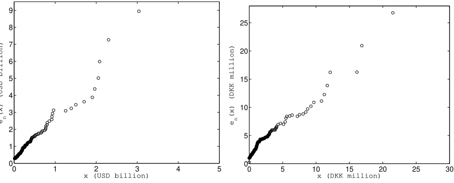
Figure 7: The empirical mean excess function ˆen(x) for the PCS catastrophe data (left panel) and the Danish fire data (right panel).

recorded by Copenhagen Re. Here we consider only losses in profits. The overall fire losses were analyzed by Embrechts, Kl¨uppelberg, and Mikosch (1997).

The Danish fire losses dataset has been already adjusted for inflation. However, the PCS dataset consists of raw data. Since the data have been collected over a considerable period of time, it is important to bring the values onto a common basis by means of a suitably chosen index. The choice of the index depends on the line of insurance. For example, an index of the cost of construction prices may be suitable for fire and other property insurance, an earnings index for life and accident insurance, and a general price index may be appropriate when a single index is required for several lines or for the whole portfolio. Here we adjust the PCS dataset using the Consumer Price Index provided by the U.S. Department of Labor. Note, that the same raw catastrophe data, however, adjusted using the discount window borrowing rate that refers to the simple interest rate at which depository institutions borrow from the Federal Reserve Bank of New York was analyzed by Burnecki, H¨ardle, and Weron (2004). A related dataset containing the national and regional PCS indices for losses resulting from catastrophic events in USA was studied by Burnecki, Kukla, and Weron (2000).

As suggested in the proceeding section we first look for the appropriate shape of the distribution. To this end we plot the empirical mean excess functions for the analyzed data sets, see Figure 7. Both in the case of PCS natural catastrophe losses and Danish fire losses the data show a super-exponential pattern suggesting a log-normal, Pareto or Burr distribution as most adequate for modeling. Hence, in the sequel we calibrate these three distributions.

We apply two estimation schemes: maximum likelihood andA2 statistics minimization. Out of the three fitted distributions only the log-normal has closed form expressions for the maximum likelihood estimators. Parameter calibration for the remaining distributions and the A2 minimization scheme is carried out via a simplex numerical optimization routine. A limited simulation study suggests that the A2 _{minimization scheme tends to return lower}

values of all edf test statistics than maximum likelihood estimation. Hence, it is exclusively used for further analysis. The results of parameter estimation and hypothesis testing for the PCS loss amounts are presented in Table 1. The Burr distribution with parametersα = 0.4801,λ = 3.9495·1016_{, andτ = 2.1524 yields the best results and}

passes all tests at the 3% level. The log-normal distribution with parametersµ=18.3806 andσ=1.1052 comes in second, however, with an unacceptable fit as tested by the Anderson-Darling statistics. As expected, the remaining distributions presented in Section 3 return even worse fits. Thus, here we suggest to choose the Burr distribution as a model for the PCS loss amounts. In the left panel of Figure 8 we present the empirical and analytical limited expected value functions for the three fitted distributions. The plot justifies the choice of the Burr distribution.

0 5 10 15 0

50 100 150 200 250 300

Analytical and empirical LEVFs (USD million) x (USD billion) 0 10 20 30 40 50 60 70

0 0.2 0.4 0.6 0.8 1 1.2

Analytical and empirical LEVFs (DKK million) x (DKK million)

Figure 8: The empirical (black solid line) and analytical limited expected value functions (LEVFs) for the log-normal (green dashed line), Pareto (blue dotted line), and Burr (red long-dashed line) distributions for the PCS catastrophe data (left panel) and the Danish fire data (right panel).

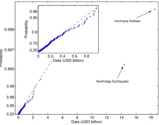
0 2 4 6 8 10 12 14 16 18

0.25 0.95 0.98 0.99 0.995 0.997 0.998

Data (USD billion)

Probability

0 0.2 0.4 0.6 0.8

0.25 0.75 0.9 0.95 0.96

Data (USD billion)

Probability

Hurricane Andrew

Northridge Earthquake

Table 1: Parameter estimates obtained via theA2_{minimization scheme and test statistics for the catastrophe loss amounts. The corresponding}

p-values based on 1000 simulated samples are given in parentheses.

Distributions: log-normal Pareto Burr

Parameters: µ=18.3806 α=3.4081 α=0.4801

σ=1.1052 λ=4.4767·108 λ=3.9495·1016

τ=2.1524

Tests: D 0.0440 0.1049 0.0366

(0.032) (<0.005) (0.072) V 0.0786 0.1692 0.0703

(0.028) (<0.005) (0.031) W2 0.1353 0.7042 0.0626

(0.012) (<0.005) (0.068) A2 1.8606 6.1160 0.5097

(<0.005) (<0.005) (0.034)

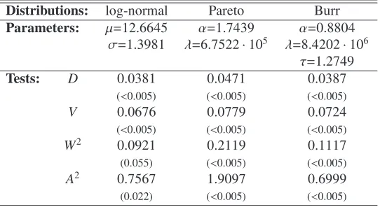
Table 2: Parameter estimates obtained via theA2_{minimization scheme and test statistics for the fire loss amounts. The correspondingp-values} based on 1000 simulated samples are given in parentheses.

Distributions: log-normal Pareto Burr

Parameters: µ=12.6645 α=1.7439 α=0.8804

σ=1.3981 λ=6.7522·105 _λ=8.4202

·106

τ=1.2749

Tests: D 0.0381 0.0471 0.0387

(<0.005) (<0.005) (<0.005) V 0.0676 0.0779 0.0724

(<0.005) (<0.005) (<0.005) W2 _{0.0921 0.2119 0.1117} (0.055) (<0.005) (<0.005) A2 _{0.7567 1.9097 0.6999} (0.022) (<0.005) (<0.005)

x1, ...,xn from the smallest to the largest: x(1) ≤... ≤ x(n) and next plotting them against their observed cumulative

frequency, i.e. the points (pluses in Fig. 9) correspond to the pairs (x(i),F−1([i−0.5]/n)), fori = 1, ...,n. If the

hypothesized distributionF(here Pareto) adequately describes the data, the plotted points fall approximately along a straight line (Burnecki and Weron, 2008). The procedure of trimming the top 1-5% of the data before calibration is known as robust estimation. Chernobai et al. (2006) showed that trimming leads to accepting the Pareto law as a model of PCS loss sizes.

References

Bratley, P., Fox, B. L., and Schrage, L. E. (1987).A Guide to Simulation, Springer-Verlag, New York.

Burnecki, K., H¨ardle, W., and Weron, R. (2004). Simulation of risk processes,inJ. Teugels, B. Sundt (eds.)Encyclopedia of Actuarial Science, Wiley, Chichester.

Burnecki, K., Kukla, G., and Weron, R. (2000). Property insurance loss distributions,Physica A287: 269-278.

Burnecki, K. and Weron, R. (2008). Visualization Tools for Insurance Risk Processes,inCh. Chen, W. H¨ardle, A. Unwin (eds.)Handbook of Data Visualization, Springer, Berlin, 899-920.

Chernobai, A., Burnecki, K., Rachev, S.T., Tr¨uck, S., and Weron, R. (2006). Modelling catastrophe claims with left-truncated severity distributions,

Computational Statistics21: 537-555.

Ciˇzek, P., H¨ardle, W., and Weron, R., eds. (2005).Statistical Tools for Finance and Insurance, Springer-Verlag, Berlin. D’Agostino, R. B. and Stephens, M. A. (1986).Goodness-of-Fit Techniques, Marcel Dekker, New York.

Daykin, C.D., Pentikainen, T., and Pesonen, M. (1994).Practical Risk Theory for Actuaries, Chapman, London. Devroye, L. (1986).Non-Uniform Random Variate Generation, Springer-Verlag, New York.

Embrechts, P., Kl¨uppelberg, C., and Mikosch, T. (1997).Modelling Extremal Events for Insurance and Finance, Springer. Hogg, R. and Klugman, S. A. (1984).Loss Distributions, Wiley, New York.

J ¨ohnk, M. D. (1964). Erzeugung von Betaverteilten und Gammaverteilten Zufallszahlen,Metrika8: 5-15. Klugman, S. A., Panjer, H.H., and Willmot, G.E. (1998).Loss Models: From Data to Decisions, Wiley, New York.

L’Ecuyer, P. (2004). Random Number Generation,inJ. E. Gentle, W. H¨ardle, Y. Mori (eds.)Handbook of Computational Statistics, Springer, Berlin, 35–70.

Panjer, H.H. and Willmot, G.E. (1992).Insurance Risk Models, Society of Actuaries, Chicago. Ross, S. (2002).Simulation, Academic Press, San Diego.

Stephens, M. A. (1978). On the half-sample method for goodness-of-fit,Journal of the Royal Statistical Society B40: 64-70.